AutoML using Pycaret

Overview

Teaching: 20 min
Exercises: 0 min

Questions

How to apply Automatic Machine Learning?

Objectives

Apply AutoML using Pycaret for regression and classification method

12a. AutoML for Regression problem

Part of this tutorial following this github

Load input data

Here, we utilize the California housing data introduced in the previous part:

import pandas as pd
import numpy as np

from sklearn.datasets import fetch_california_housing
from sklearn.model_selection import train_test_split

data = fetch_california_housing()

# Predictors/Input:
X = pd.DataFrame(data.data,columns=data.feature_names)

# Predictand/output:
y = pd.DataFrame(data.target,columns=data.target_names)

# Merge X and y into 1 set of data:
d_data = X.join(y)

Split data into training/testing/validation

We split the entire data with 90% for training/validation and 10% for testing/unseen

# 90% data for training/testing and 10% for validation

data_traintest = d_data.sample(frac=0.9, random_state=123)
data_unseen = d_data.drop(data_traintest.index)

data_traintest.reset_index(drop=True, inplace=True)
data_unseen.reset_index(drop=True, inplace=True)

print('Data for Modeling: ' + str(data_traintest.shape))
print('Unseen Data For Predictions: ' + str(data_unseen.shape))

Split data for train/test with random state and 70% for training

d_train, d_test = train_test_split(data_traintest, random_state =123 , test_size = 0.3)

Apply Pycaret for AutoML

Note that in data, we already merge the y which is “MedHouseVal” to entire data set so the code below will pull out the target price:

from pycaret.regression import *
setup_df = setup(data= d_train, target = 'MedHouseVal',html=False, silent=True, verbose=False)

Comparing all models:

Comparing all models to evaluate performance is the recommended starting point for modeling once the setup is completed (unless you exactly know what kind of model you need, which is often not the case). This function trains all models in the model library and scores them using k-fold cross validation for metric evaluation. The output prints a score grid that shows average MAE, MSE, RMSE, R2, RMSLE and MAPE accross the folds (10 by default) along with training time.

best=compare_models()

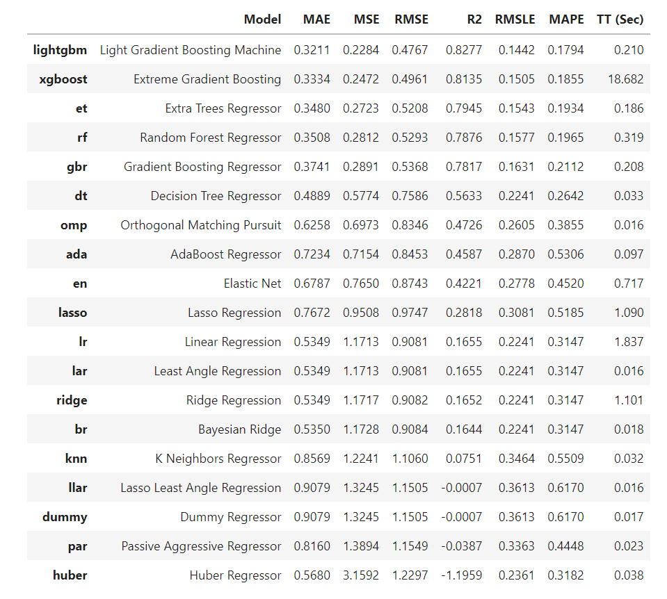
Two simple lines of code have trained and evaluated over 20 models using cross validation. The score grid printed above highlights the highest performing metric for comparison purposes only. The grid by default is sorted using R2 (highest to lowest) which can be changed by passing sort parameter. For example compare_models(sort = ‘RMSE’) will sort the grid by RMSE (lower to higher since lower is better). If you want to change the fold parameter from the default value of 10 to a different value then you can use the fold parameter. For example compare_models(fold = 5) will compare all models on 5 fold cross validation. Reducing the number of folds will improve the training time. By default, compare_models return the best performing model based on default sort order but can be used to return a list of top N models by using n_select parameter.

Create Model

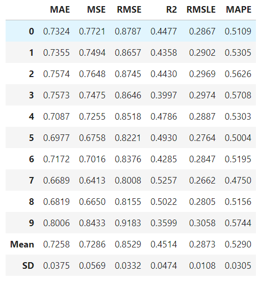
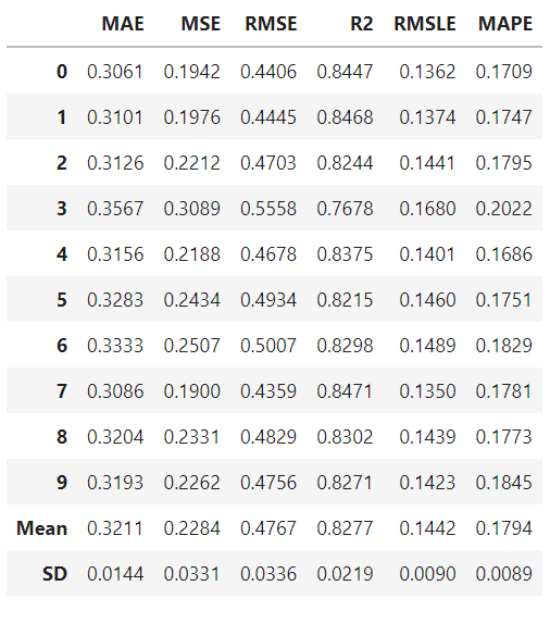
create_model is the most granular function in PyCaret and is often the foundation behind most of the PyCaret functionalities. As the name suggests this function trains and evaluates a model using cross validation that can be set with fold parameter. The output prints a score grid that shows MAE, MSE, RMSE, R2, RMSLE and MAPE by fold.

For the remaining part of this tutorial, we will work with the below models as our candidate models. The selections are for illustration purposes only and do not necessarily mean they are the top performing or ideal for this type of data.

Ada (‘ada’)
Light Gradient Boosting Machine (‘lightgbm’)
Decision Tree (‘dt’)

There are 25 regressors available in the model library of PyCaret. To see list of all regressors either check the docstring or use models function to see the library.

models()

Create Adaptive Boosting Model

ada = create_model('ada')

Create Light Gradient Boosting Model

lightgbm = create_model('lightgbm')

Create Decision Tree Model

dt = create_model("dt")

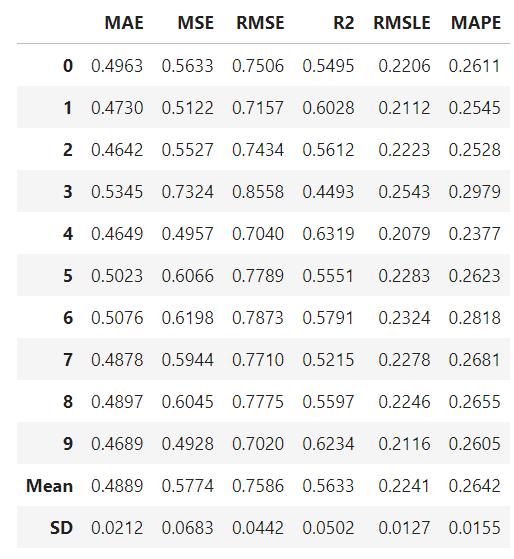
Notice that the Mean score of all models matches with the score printed in compare_models(). This is because the metrics printed in the compare_models() score grid are the average scores across all CV folds. Similar to compare_models(), if you want to change the fold parameter from the default value of 10 to a different value then you can use the fold parameter. For Example: create_model(‘rf’, fold = 5) to create Random Forest using 5 fold cross validation.

Tune a model

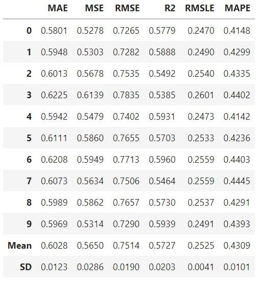
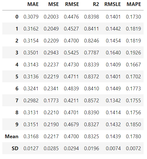
When a model is created using the create_model function it uses the default hyperparameters to train the model. In order to tune hyperparameters, the tune_model function is used. This function automatically tunes the hyperparameters of a model using Random Grid Search on a pre-defined search space. The output prints a score grid that shows MAE, MSE, RMSE, R2, RMSLE and MAPE by fold. To use the custom search grid, you can pass custom_grid parameter in the tune_model function (see 9.2 LightGBM tuning below).

Adaboost

tuned_ada = tune_model(ada)

Light GBM

lgbm_params = {'num_leaves': np.arange(10,200,10),
                        'max_depth': [int(x) for x in np.linspace(10, 110, num = 11)],
                        'learning_rate': np.arange(0.1,1,0.1)
                        }
tuned_lightgbm = tune_model(lightgbm)                        

Decision Tree

tuned_dt = tune_model(dt)

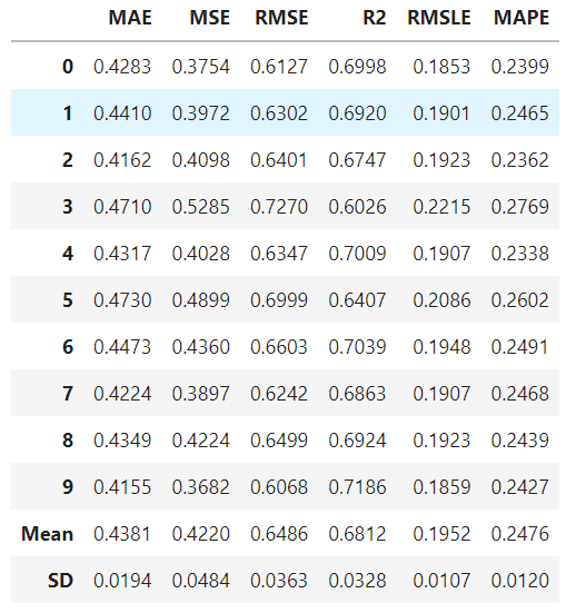
By default, tune_model optimizes R2 but this can be changed using optimize parameter. For example: tune_model(dt, optimize = ‘MAE’) will search for the hyperparameters of a Decision Tree Regressor that results in the lowest MAE instead of highest R2. For the purposes of this example, we have used the default metric R2 for the sake of simplicity only. The methodology behind selecting the right metric to evaluate a regressor is beyond the scope of this tutorial but if you would like to learn more about it, you can click here to develop an understanding on regression error metrics.

Metrics alone are not the only criteria you should consider when finalizing the best model for production. Other factors to consider include training time, standard deviation of k-folds etc. As you progress through the tutorial series we will discuss those factors in detail at the intermediate and expert levels. For now, let’s move forward considering the Tuned Light Gradient Boosting Machine stored in the tuned_lightgbm variable as our best model for the remainder of this tutorial.

Plot model

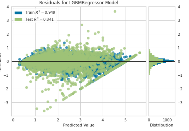
Before model finalization, the plot_model() function can be used to analyze the performance across different aspects such as Residuals Plot, Prediction Error, Feature Importance etc. This function takes a trained model object and returns a plot based on the test / hold-out set.

There are over 10 plots available, please see the plot_model() docstring for the list of available plots.

Residual Plot

plot_model(tuned_lightgbm)

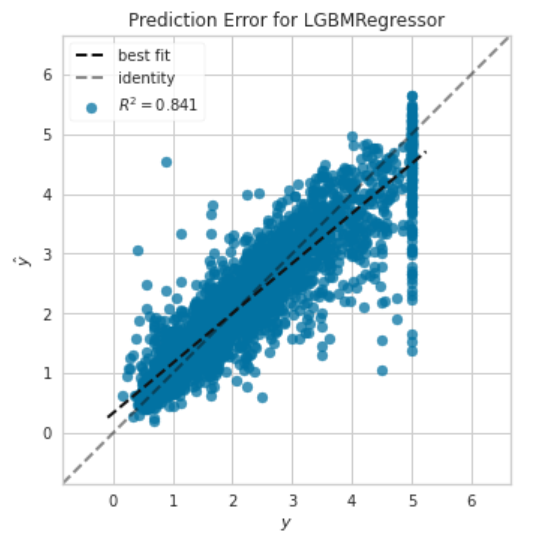
Predicted error plot

plot_model(tuned_lightgbm, plot = 'error')

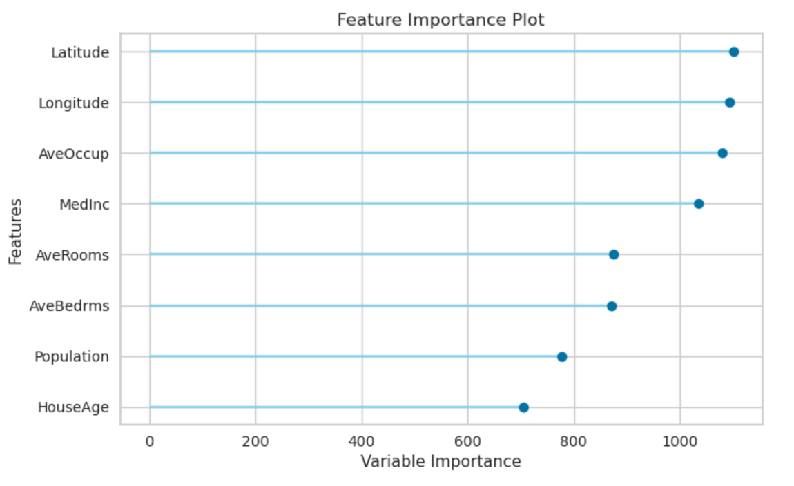
Feature Important Plot

plot_model(tuned_lightgbm, plot='feature')

Predict on Test / Hold-out Sample

Before finalizing the model, it is advisable to perform one final check by predicting the test/hold-out set and reviewing the evaluation metrics. If you look at the information grid in Section 6 above, you will see that 30% (1621 samples) of the data has been separated out as a test/hold-out sample. All of the evaluation metrics we have seen above are cross-validated results based on training set (70%) only. Now, using our final trained model stored in the tuned_lightgbm variable we will predict the hold-out sample and evaluate the metrics to see if they are materially different than the CV results.m

predict_model(tuned_lightgbm);

The R2 on the test/hold-out set is 0.8414 compared to 0.8325 mean achieved on tuned_lightgbm CV results. This is not a significant difference. If there is a large variation between the test/hold-out and CV results, then this would normally indicate over-fitting but could also be due to several other factors and would require further investigation. In this case, we will move forward with finalizing the model and predicting on unseen data (the 10% that we had separated in the beginning and never exposed to PyCaret).

(TIP : It’s always good to look at the standard deviation of CV results when using create_model.)

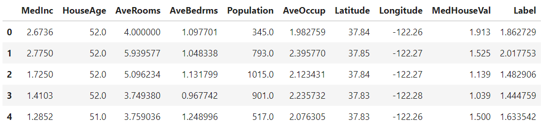
Predict on Unseen data

final_lightgbm = finalize_model(tuned_lightgbm)

unseen_predictions = predict_model(final_lightgbm, data=data_unseen)
unseen_predictions.head()

12b. AutoML for Classification problem with multiple output

The material following this pycaret tutorial on github

Here we utilize the renown iris dataset as an example for the AutoML using pycaret.

from pycaret.datasets import get_data
dataset = get_data('iris')

Split training/testing & unseen data

data = dataset.sample(frac=0.9, random_state=123)
data_unseen = dataset.drop(data.index)

data.reset_index(drop=True, inplace=True)
data_unseen.reset_index(drop=True, inplace=True)

print('Data for Modeling: ' + str(data.shape))
print('Unseen Data For Predictions: ' + str(data_unseen.shape))

Data for Modeling: (135, 5) Unseen Data For Predictions: (15, 5)

Setting up the model and compare all of them

Comparing all models to evaluate performance is the recommended starting point for modeling once the setup is completed (unless you exactly know what kind of model you need, which is often not the case). This function trains all models in the model library and scores them using stratified cross validation for metric evaluation. The output prints a score grid that shows average Accuracy, Recall, Precision, F1, Kappa, and MCC accross the folds (10 by default) along with training times.

best = compare_models()

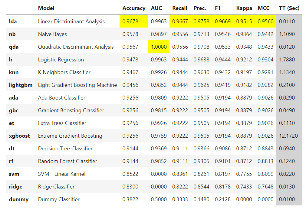
Two simple words of code (not even a line) have trained and evaluated over 15 models using cross validation. The score grid printed above highlights the highest performing metric for comparison purposes only. The grid by default is sorted using ‘Accuracy’ (highest to lowest) which can be changed by passing the sort parameter. For example compare_models(sort = ‘Recall’) will sort the grid by Recall instead of Accuracy. If you want to change the fold parameter from the default value of 10 to a different value then you can use the fold parameter. For example compare_models(fold = 5) will compare all models on 5 fold cross validation. Reducing the number of folds will improve the training time. By default, compare_models return the best performing model based on default sort order but can be used to return a list of top N models by using n_select parameter.

Note: The AUC metric is not available for Multiclass classification however the column will still be shown with zero values to maintain consistency between the Binary Classification and Multiclass Classification display grids.

Create 3 models

Decision Tree Classifier (‘dt’)
K Neighbors Classifier (‘knn’)
Logistic Regression (‘lr’)

There are 18 classifiers available in the model library of PyCaret. Please view the create_model() docstring for the list of all available models.

dt = create_model('dt')
knn = create_model('knn')
lr = create_model('lr')

Notice that the Mean score of all models matches with the score printed in compare_models(). This is because the metrics printed in the compare_models() score grid are the average scores across all CV folds. Similar to compare_models(), if you want to change the fold parameter from the default value of 10 to a different value then you can use the fold parameter. For Example: create_model(‘dt’, fold = 5) will create a Decision Tree Classifier using 5 fold stratified CV.

Tune these 3 models

When a model is created using the create_model() function it uses the default hyperparameters to train the model. In order to tune hyperparameters, the tune_model() function is used. This function automatically tunes the hyperparameters of a model using Random Grid Search on a pre-defined search space. The output prints a score grid that shows Accuracy, AUC, Recall, Precision, F1, Kappa, and MCC by fold for the best model. To use the custom search grid, you can pass custom_grid parameter in the tune_model function (see 9.2 KNN tuning below).

tuned_dt = tune_model(dt)
tuned_knn = tune_model(knn, custom_grid = {'n_neighbors' : np.arange(0,50,1)})
tuned_lr = tune_model(lr)

The tune_model() function is a random grid search of hyperparameters over a pre-defined search space. By default, it is set to optimize Accuracy but this can be changed using the optimize parameter. For example: tune_model(dt, optimize = ‘Recall’) will search for the hyperparameters of a Decision Tree Classifier that result in the highest Recall. For the purposes of this example, we have used the default metric Accuracy for the sake of simplicity only. The methodology behind selecting the right metric to evaluate a classifier is beyond the scope of this tutorial but if you would like to learn more about it, you can click here to read an article on how to choose the right evaluation metric.

Metrics alone are not the only criteria you should consider when finalizing the best model for production. Other factors to consider include training time, standard deviation of kfolds etc. As you progress through the tutorial series we will discuss those factors in detail at the intermediate and expert levels. For now, let’s move forward considering the Tuned K Neighbors Classifier as our best model for the remainder of this tutorial.

Plot models

Before model finalization, the plot_model() function can be used to analyze the performance across different aspects such as AUC, confusion_matrix, decision boundary etc. This function takes a trained model object and returns a plot based on the test / hold-out set.

There are 15 different plots available, please see the plot_model() docstring for the list of available plots.

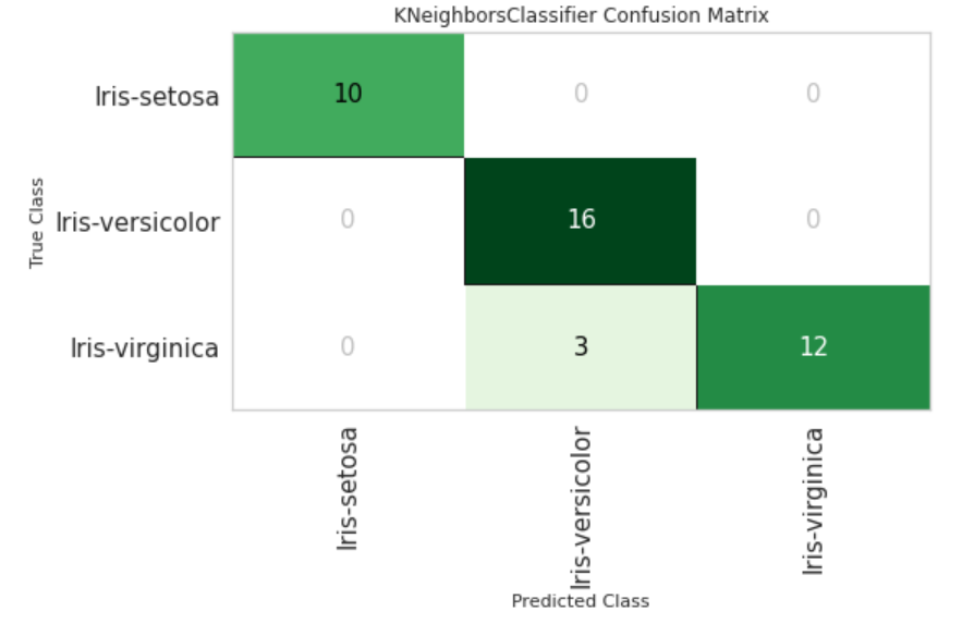
Plotting confusion matrix

Sample plot using tuned_knn model

plot_model(tuned_knn, plot = 'confusion_matrix')

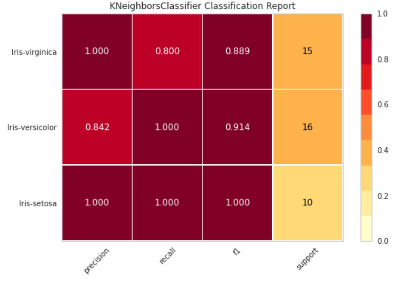
Classication report

Get the class report for tuned_knn model

plot_model(tuned_knn, plot = 'class_report')

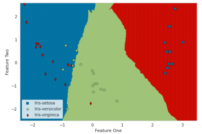
Decision Boundary

Plot the decision boundary for tuned_knn model

plot_model(tuned_knn, plot='boundary')

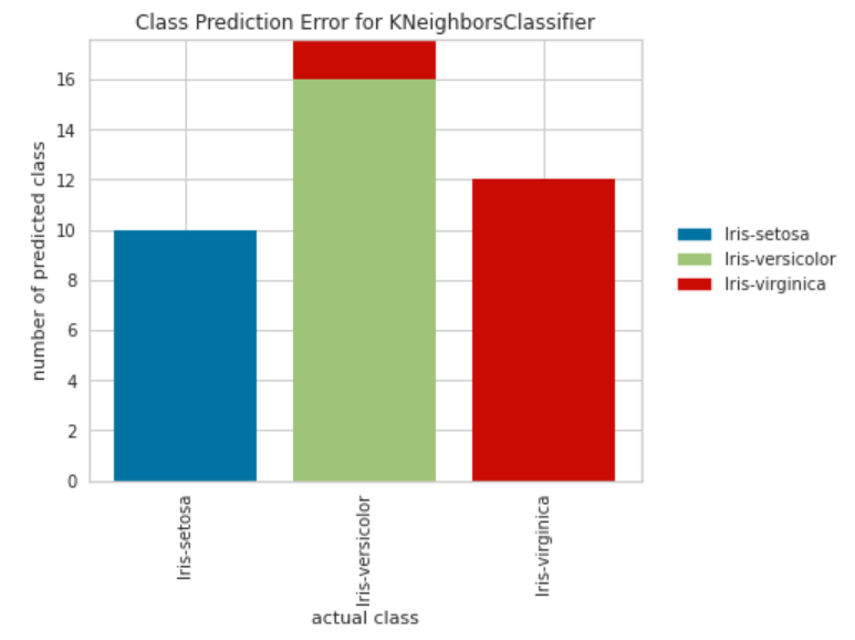
Prediction Error

Plot the prediction error for tuned_knn model

plot_model(tuned_knn, plot = 'error')

Evaluate the model

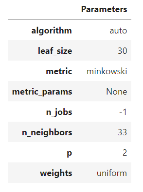
Another way to analyze the performance of models is to use the evaluate_model() function which displays a user interface for all of the available plots for a given model. It internally uses the plot_model() function.

evaluate_model(tuned_knn)

Predict on test / hold-out Sample

Before finalizing the model, it is advisable to perform one final check by predicting the test/hold-out set and reviewing the evaluation metrics. If you look at the information grid in Section 6 above, you will see that 30% (41 samples) of the data has been separated out as a test/hold-out sample. All of the evaluation metrics we have seen above are cross validated results based on the training set (70%) only. Now, using our final trained model stored in the tuned_knn variable we will predict against the hold-out sample and evaluate the metrics to see if they are materially different than the CV results.

predict_model(tuned_knn)

The accuracy on the test/hold-out set is 0.9512 compared to 0.9356 achieved on the tuned_knn CV results (in section 9.2 above). This is not a significant difference. If there is a large variation between the test/hold-out and CV results, then this would normally indicate over-fitting but could also be due to several other factors and would require further investigation. In this case, we will move forward with finalizing the model and predicting on unseen data (the 10% that we had separated in the beginning and never exposed to PyCaret).

(TIP : It’s always good to look at the standard deviation of CV results when using create_model().)

Finalize Model for Deployment

Model finalization is the last step in the experiment. A normal machine learning workflow in PyCaret starts with setup(), followed by comparing all models using compare_models() and shortlisting a few candidate models (based on the metric of interest) to perform several modeling techniques such as hyperparameter tuning, ensembling, stacking etc. This workflow will eventually lead you to the best model for use in making predictions on new and unseen data. The finalize_model() function fits the model onto the complete dataset including the test/hold-out sample (30% in this case). The purpose of this function is to train the model on the complete dataset before it is deployed in production.

final_knn = finalize_model(tuned_knn)

Predict on unseen data

The predict_model() function is also used to predict on the unseen dataset. The only difference from section 11 above is that this time we will pass the data_unseen parameter. data_unseen is the variable created at the beginning of the tutorial and contains 10% (15 samples) of the original dataset which was never exposed to PyCaret. (see section 5 for explanation)

unseen_predictions = predict_model(final_knn, data=data_unseen)
unseen_predictions.head()

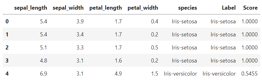
The Label and Score columns are added onto the data_unseen set. Label is the prediction and score is the probability of the prediction. Notice that predicted results are concatenated to the original dataset while all the transformations are automatically performed in the background.

Key Points

Kaggle

previous episode

Introduction to Machine Learning using Python

next episode