Overview

Teaching: 20 min
Exercises: 0 min

Questions

• How to train a Machine Learning model with continuos output

Objectives

• Learn to use different ML algorithm for Supervised Learning

5 Supervised Learning with continuous output

For this session, we gonna use several Machine Learning algorithm to work with continuous output the supervised learning problem. First of all, let’s import the data:

5.1 Preprocessing

5.1.1 Import data

Let use the california housing data in previous episodes:

import pandas as pd
import numpy as np

from sklearn.datasets import fetch_california_housing

data = fetch_california_housing()

# Predictors/Input:
X = pd.DataFrame(data.data,columns=data.feature_names)

# Predictand/output:
y = pd.DataFrame(data.target,columns=data.target_names)

print(X.head())
print(y.head())

5.1.2 Check missing data

print(X.isnull().sum())
print(y.isnull().sum())

Since there is no missing data, we move on to the next step:

5.1.3 Split model into training & testing set with 60% for training:

from sklearn.model_selection import train_test_split
X_train, X_test, y_train, y_test = train_test_split(X,y,train_size=0.6,random_state=123)

5.1.4 Visualization the inputs and output:

We can visualize the inputs and output data using pair plotting with seaborn package.

Make sure that you install seaborn package in advance (Open the ML_SKLN Console (Not Notebook) and run this command:)

pip install seaborn

Once seaborn is installed, you can plot visualize the input/output data:

df = pd.concat([X_train,y_train], axis=1)
sns.pairplot(df)

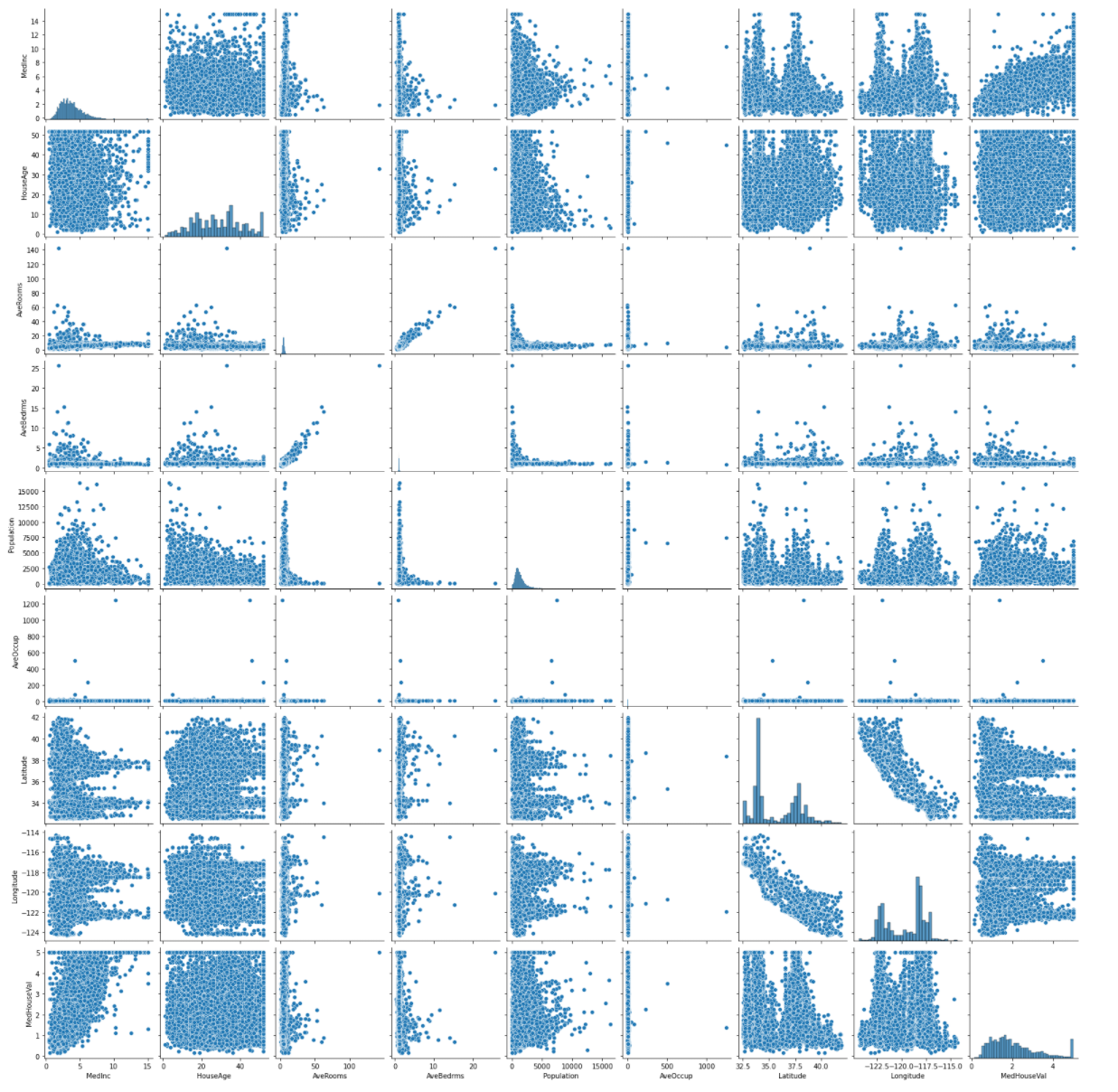
Now the input data is ready for supervised learning model, let’s select several ML algorithms to work with:

5.2 Machine Learning algorithm with Linear Regression

5.2.1 Train model using Linear Regression with 1 predictor (for example Medium Income)

Fit a Linear model using LinearRegression model:

from sklearn.linear_model import LinearRegression
model_linreg1 = LinearRegression().fit(pd.DataFrame(X_train['MedInc']),y_train)

Apply trained model to testing data set and evaluate output using R-squared:

from sklearn import metrics
y_pred = model_linreg1.predict(pd.DataFrame(X_test['MedInc']))
print("R2 is: %1.2f" % metrics.r2_score(y_test,y_pred)) 
print("RMSE is: %1.2f" % metrics.mean_squared_error(y_test,y_pred,squared=False)) 

the result is:

R2 is: 0.48
RMSE is: 0.84

We see that using 1 predictor/input, we obtain the output with corresponding R2 of 0.48 and RMSE = 0.84, which is not good enough. (The good R2 should be more than 0.7) Therefore, we change the approach, still using Linear Regression but with more inputs:

5.2.2 Train model using Multi-Linear Regression (with 2 or more predictors)

In this section, we will build the model with 4 inputs [“MedInc”,”HouseAge”,”AveRooms”,”Population”]

Fit the training set and predict using test set

model_linreg = LinearRegression().fit(X_train[["MedInc","HouseAge","AveRooms","Population"]],y_train)
y_pred2 = model_linreg.predict(X_test[["MedInc","HouseAge","AveRooms","Population"]])

print("R2 is: %1.2f" % metrics.r2_score(y_test,y_pred2))
print("RMSE is: %1.2f"  % metrics.mean_squared_error(y_test,y_pred2,squared=False)) 

Output is therefore better with smaller RMSE and higher Rsquared:

R2 is: 0.52
RMSE is: 0.80

Still the model outcome is not good enough, so we try another algorithm:

5.2.3 Train model using Polynomial Regression

We can slightly improve this by using Polynomial Regression

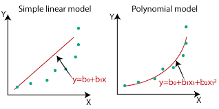
Preprocessing: polynomial regression with degree of freedom=2

the degree-2 polynomial features for 2 inputs (a & b) are [1, a, b, a^2, ab, b^2].

from sklearn.preprocessing import PolynomialFeatures
poly = PolynomialFeatures(degree=2)
X_poly = poly.fit_transform(X[["MedInc","HouseAge","AveRooms","Population"]])

X_train, X_test, y_train, y_test = train_test_split(pd.DataFrame(X_poly),y, train_size=0.6,random_state=123)

print(X_poly.shape)

We see that using 4 inputs data, with Polynomial regression, we have 15 input variables [1 a b c d a2 ab ac ad b2 bc bd c2 cd d2]

Fit the new dataset and predict output:

model_linreg_poly = LinearRegression().fit(X_train,y_train)
y_pred_poly = model_linreg_poly.predict(X_test)

print("R2 is: %1.2f " % metrics.r2_score(y_test,y_pred_poly)) 
print("RMSE is: %1.2f" % metrics.mean_squared_error(y_test,y_pred_poly,squared=False))

The output is even better with R2 for testing data is 0.55 and lower RMSE.

R2 is: 0.55 
RMSE is: 0.78

The R2=0.55 shows improvement using polynomial regression!

How about using more degrees of freedom?

Polynomial regression with degree of freedom=4

Can we improve the result with more degree of freedome? Let’s try using df=4:

from sklearn.preprocessing import PolynomialFeatures
poly = PolynomialFeatures(degree=4)
X_poly = poly.fit_transform(X[["MedInc","HouseAge","AveRooms","Population"]])

X_train4, X_test4, y_train4, y_test4 = train_test_split(pd.DataFrame(X_poly),y, train_size=0.6,random_state=123)

model_linreg_poly4 = LinearRegression().fit(X_train4,y_train4)
y_pred_poly4 = model_linreg_poly4.predict(X_test4)

print("R2 for 4 dof is: %1.2f " % metrics.r2_score(y_test4,y_pred_poly4)) 
print("RMSE for 4 dof is: %1.2f" % metrics.mean_squared_error(y_test4,y_pred_poly4,squared=False)) 

the output is:

R2 for 4 dof of testing is: -4.33 
RMSE for 4 dof of testing is: 2.68

The R2 in sklearn can be negative, it arbitrarily means that the model is worse. More info on sklearn r2_score.

Why increasing the degree of freedom, my results getting worst? It’s called OVERFITTING

5.3 Overfitting

Overfitting occurs when we used lots of unesscessary input data for training process. It fits the training data so well that it is worse when applied to testing data:

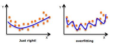
Exercise 1: Let use all dataset to train the data to see if using all input data, we have overfitting?

Exercise 2: Let’s check the R2 and RMSE for training set using 2 and 4 degree of freedom to see if the 4 dof is better than 2 dof in fitting back to training data?

5.4 Other Supervised ML algorithm for continuous data

There are many other ML algorithm that helps to overcome the issue of overfitting, for example:

5.4.1 Decision Tree

• Tree based learning algorithms are considered to be one of the best and mostly used supervised learning methods.
• Tree based methods empower predictive models with high accuracy, stability and ease of interpretation
• Non-parametric and non-linear relationships
• Types: Continuous (DecisionTreeRegressor) and Categorical (DecisionTreeClassifier)

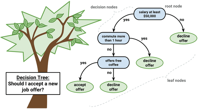
Let use all data in this exercise, the Decision Tree algorithm for continuous output in sklearn is called DecisionTreeRegressor

X_train, X_test, y_train, y_test = train_test_split(X,y,train_size=0.6,random_state=123)

from sklearn.tree import DecisionTreeRegressor
model_DT = DecisionTreeRegressor(max_depth=4).fit(X_train,y_train)
y_pred_DT = model_DT.predict(X_test)

print("R2 using Decision Tree is: %1.2f " % metrics.r2_score(y_test,y_pred_DT)) 
print("RMSE using Decision Tree is: %1.2f" % metrics.mean_squared_error(y_test,y_pred_DT,squared=False))

output:

R2 using Decision Tree is: 0.58 
RMSE using Decision Tree is: 0.76

Now we can see that Decision Tree helps to overcome the overfitting by trimming down the unnecessary input data.

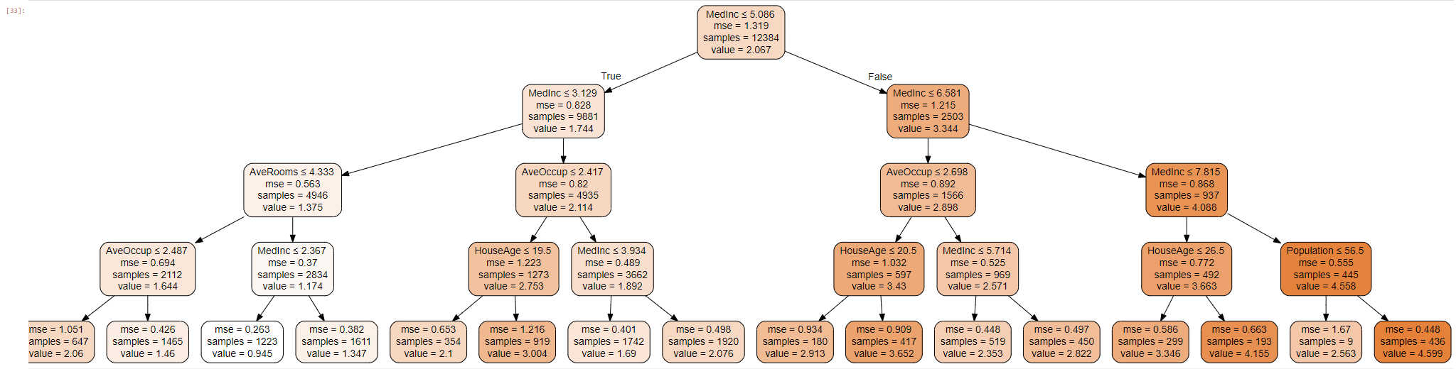
Visualization the Decision Tree:

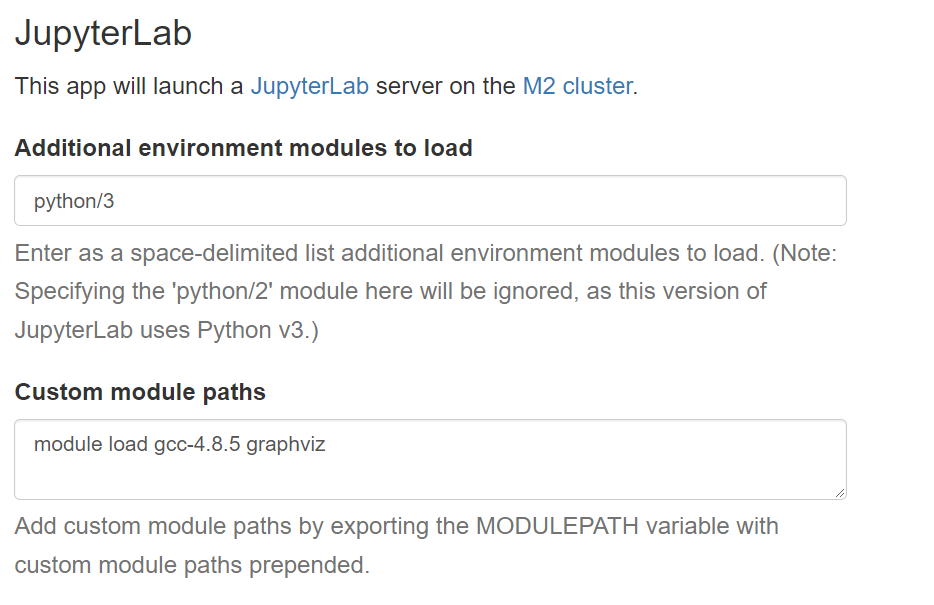
The following required graphviz model to be loaded when you requested for a Python Notebook.

from sklearn import tree
import graphviz
dot_data = tree.export_graphviz(model_DT, out_file=None,                      
                      filled=True, rounded=True,
                      feature_names=data.feature_names,
                      special_characters=True)  
graph = graphviz.Source(dot_data) 
graph

5.4.2 Random Forest

• Random Forest is considered to be a panacea of all data science problems. On a funny note, when you can’t think of any algorithm (irrespective of situation), use random forest!
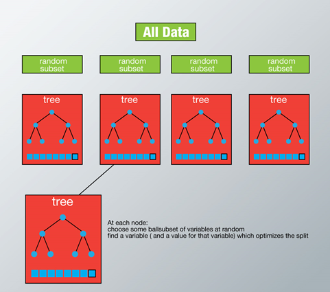
• Opposite to Decision Tree, Random Forest use bootstrapping technique to grow multiple tree
• Random Forest is a versatile machine learning method capable of performing both regression and classification tasks.
• It is a type of ensemble learning method, where a group of weak models combine to form a powerful model.
• The end output of the model is like a black box and hence should be used judiciously.

from sklearn.ensemble import RandomForestRegressor
model_RF = RandomForestRegressor(n_estimators=10).fit(X_train,y_train)
y_pred_RF = model_RF.predict(X_test)

print("R2 using Random Forest is: %1.2f " % metrics.r2_score(y_test,y_pred_RF)) 
print("RMSE using Random Forest is: %1.2f" % metrics.mean_squared_error(y_test,y_pred_RF,squared=False))

Here we use n=10 estimators (growing using n trees in the forest) and The output is much better:

R2 using Random Forest is: 0.81 
RMSE using Random Forest is: 0.51

5.5 Ensemble Machine Learning

• Ensemble is a method in Machine Learning that combine decision from several ML models to obtain optimum output.
• Ensemble methods use multiple learning algorithms to obtain better predictive performance than could be obtained from any of the constituent learning algorithms alone. Unlike a statistical ensemble in statistical mechanics, which is usually infinite, a machine learning ensemble consists of only a concrete finite set of alternative models, but typically allows for much more flexible structure to exist among those alternatives
• The bonus point when applying both Bagging and Boosting in sklearn that they can be run in parallel!

Types of Ensembles:

There are 2 main types of Ensembles in ML:

Bagging: Boostrap Aggregation

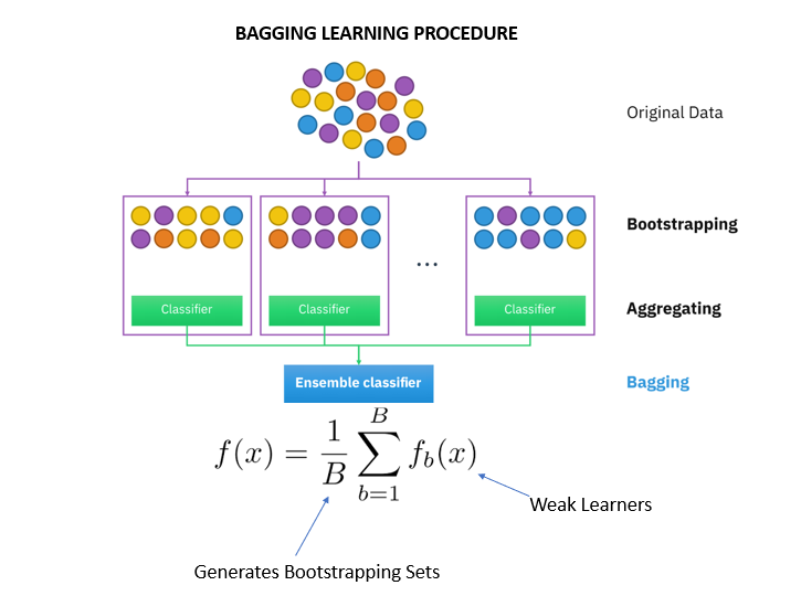
• Bagging, also known as bootstrap aggregation, is the ensemble learning method that is commonly used to reduce variance within a noisy dataset.
• In bagging, a random sample of data in a training set is selected with replacement—meaning that the individual data points can be chosen more than once.

• After several data samples are generated, these weak models are then trained independently, and depending on the type of task—regression or classification, for example—the average or majority of those predictions yield a more accurate estimate.

• As a note, the Random Forest algorithm is considered an extension of the bagging method, using both bagging and feature randomness to create an uncorrelated forest of decision trees.

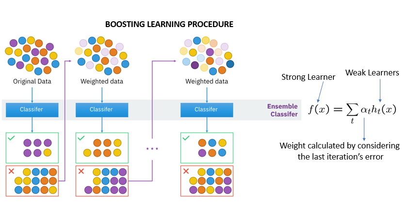
Boosting: Boost the weak predictors

• Boosting is an ensemble learning method that combines a set of weak learners into a strong learner to minimize training errors.
• In boosting, a random sample of data is selected, fitted with a model and then trained sequentially—that is, each model tries to compensate for the weaknesses of its predecessor.
• With each iteration, the weak rules from each individual classifier are combined to form one, strong prediction rule.

5.5.1 Bagging with RandomForest

We can apply Bagging to different ML algorithm like Linear Regression, Decision Tree, Random Forest, etc. Following are the syntax:

from sklearn.ensemble import BaggingRegressor, RandomForestRegressor

model_RF = RandomForestRegressor()

model_bag_RF = BaggingRegressor(base_estimator=model_RF, n_estimators=100,
                            bootstrap=True, n_jobs=-1,
                            random_state=123)
                            
model_bag_RF.fit(X_train, y_train)

y_pred_bagRF = model_bag_RF.predict(X_test)

print("R2 using Bagging Random Forest is: %1.2f " % metrics.r2_score(y_test,y_pred_bagRF)) 
print("RMSE using Baggin Random Forest is: %1.2f" % metrics.mean_squared_error(y_test,y_pred_bagRF,squared=False))

Note that here we use n_estimators = 100 for bagging model (it grows 100 times the RandomForest model). The n_jobs=-1 means that it utilizes all the cores inside a compute nodes that we have

And the output is very similar to RandomForest:

R2 using Bagging Random Forest is: 0.80 
RMSE using Baggin Random Forest is: 0.51

Let’s try with some Boosting Ensemble approach:

5.5.2 Boosting with Adaboost

A single classifier may not be able to accurately predict the class of an object, but when we group multiple weak classifiers with each one progressively learning from the others’ wrongly classified objects, we can build one such strong model.

A weak classifier is one that performs better than random guessing, but still performs poorly at designating classes to objects.

To understand more about Adaboost, you are encouraged to read here

from sklearn.ensemble import AdaBoostRegressor
model_ADA = AdaBoostRegressor(n_estimators=100, learning_rate=0.03).fit(X_train, y_train)
y_pred_ADA = model_ADA.predict(X_test)

print("R2 using Adaboost is: %1.2f " % metrics.r2_score(y_test,y_pred_ADA)) 
print("RMSE using Adaboost is: %1.2f" % metrics.mean_squared_error(y_test,y_pred_ADA,squared=False))

The output is not as good as Bagging RF

R2 using Adaboost is: 0.59 
RMSE using Adaboost is: 0.75

5.5.3 Gradient Boosting Machine

Gradient Boosting trains many models in a gradual, additive and sequential manner. The major difference between AdaBoost and Gradient Boosting Algorithm is how the two algorithms identify the shortcomings of weak learners (eg. decision trees). While the AdaBoost model identifies the shortcomings by using high weight data points, gradient boosting performs the same by using gradients in the loss function (y=ax+b+e , e needs a special mention as it is the error term). More information can be found here

from sklearn.ensemble import GradientBoostingRegressor
model_GBM = GradientBoostingRegressor(n_estimators=100).fit(X_train,y_train)
y_pred_GBM = model_GBM.predict(X_test)

print("R2 using GBM is: %1.2f " % metrics.r2_score(y_test,y_pred_GBM)) 
print("RMSE using GBM is: %1.2f" % metrics.mean_squared_error(y_test,y_pred_GBM,squared=False))

The output is better than Adaboost:

R2 using GBM is: 0.79 
RMSE using GBM is: 0.53

Which is better in Ensemble? Bagging or Boosting?

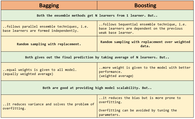
• Ensemble overcome the limitation of using only single model
• Between bagging and boosting, there is no better approach without trial & error.

Key Points

• Supervised Learning with continuous output