Overview

Teaching: 20 min
Exercises: 0 min

Questions

• How to train a Machine Learning model with Categorical output?

Objectives

• Learn different ML Supervised Learning with Categorical output

6 Supervised Learning with categorical output

• Typical Classification problem with 2, 3, 4 (or more) outputs.
• Most of the time the output consists of binary (male/female, spam/nospam,yes/no)
• Sometime, there are more than binary output: dog/cat/mouse, red/green/yellow.

In this category, we gonna use 2 existing dataset from sklearn:

• Breast Cancer Wisconsine data for Binary output
• Iris plant data for multiple (3) output.

6.1 Logistic Regression for binary output

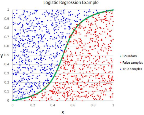
• Logistic regression is another technique borrowed by machine learning from the field of statistics. It is the go-to method for binary classification problems (problems with two class values).
• Typical binary classification: True/False, Yes/No, Pass/Fail, Spam/No Spam, Male/Female
• Unlike linear regression, the prediction for the output is transformed using a non-linear function called the logistic function.
• The standard logistic function has formulation:

In this example, we load a sample dataset called Breast Cancer Wisconsine.

Load Breast Cancer Wisconsine data

from sklearn.datasets import load_breast_cancer

data = load_breast_cancer()
X = data.data
y = data.target
print("There are", X.shape[1], " Predictors: ", data.feature_names)
print("The output has 2 values: ", data.target_names)
print("Total size of data is ", X.shape[0], " rows")

We can see that there are 30 input data representing the shape and size of 569 tumours. Base on that, the tumour can be considered malignant or benign (0 or 1 as in number)

Partitioning Data to train/test:

from sklearn.model_selection import train_test_split
X_train, X_test, y_train, y_test = train_test_split(X, y, test_size=0.6, random_state=123)

Train model using Logistic Regression

For simplicity, we use all predictors for the regression:

from sklearn.linear_model import LogisticRegression
model_LogReg = LogisticRegression(solver='newton-cg').fit(X_train, y_train)

Evaluate model output:

y_pred = model_LogReg.predict(X_test)

from sklearn import metrics
print("The accuracy score is %1.3f" % metrics.accuracy_score(y_test,y_pred))

We retrieve the accuracy = 0.965 using all predictors

Compute AUC-ROC and plot curve

from sklearn.metrics import roc_curve, roc_auc_score
import matplotlib.pyplot as plt
import numpy as np

lr_probs = model_LogReg.predict_proba(X_test)
# generate a no skill prediction (majority class)
ns_probs = np.zeros(len(y_test))

# calculate scores
ns_auc = roc_auc_score(y_test, ns_probs)
lr_auc = roc_auc_score(y_test, lr_probs[:,1])
# summarize scores
print('No Skill: ROC AUC=%.3f' % (ns_auc))
print('Logistic: ROC AUC=%.3f' % (lr_auc))
# calculate roc curves
ns_fpr, ns_tpr, _ = roc_curve(y_test, ns_probs)
lr_fpr, lr_tpr, _ = roc_curve(y_test, lr_probs[:,1])
# plot the roc curve for the model
plt.plot(ns_fpr, ns_tpr, linestyle='--', label='No Skill')
plt.plot(lr_fpr, lr_tpr, marker='.', label='Logistic')
# axis labels
plt.xlabel('False Positive Rate')
plt.ylabel('True Positive Rate')
# show the legend
plt.legend()
# show the plot
plt.show()

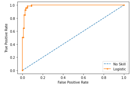
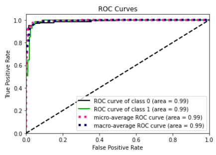
An alternative way to plot AUC-ROC curve, using additional toolbox “scikit-plot”

pip install scikit-plot

The shorter code for using this library:

import scikitplot as skplt
skplt.metrics.plot_roc(y_test, lr_probs)
plt.show()

6.2 Classification problem with more than 3 outputs

Here we use Iris plant data for multiple (3) output.

Import data

from sklearn.datasets import load_iris
data = load_iris()
X = data.data
y = data.target

print("There are", X.shape[1], " Predictors: ", data.feature_names)
print("The output has 3 values: ", data.target_names)
print("Total size of data is ", X.shape[0], " rows")

• We can see that there are 4 input data representing the petal/sepal width and length of 3 different kind of iris flowers.
• Base on that, the iris plants can be classified as ‘setosa’ ‘versicolor’ ‘virginica’.

Partitioning Data to train/test:

from sklearn.model_selection import train_test_split
X_train, X_test, y_train, y_test = train_test_split(X, y, test_size=0.6, random_state=123)

Train model using Linear Discriminant Analysis (LDA):

For simplicity, we use all predictors for the regression:

from sklearn.discriminant_analysis import LinearDiscriminantAnalysis
model_LDA = LinearDiscriminantAnalysis().fit(X_train,y_train)

Evaluate model output:

print("The accuracy score is %1.3f" % model_LDA.score(X_test,y_test))

LDA can be used for both binary and more categorical output

Exercise: create an LDA model to predict the breast cancer Wisconsine data

6.3 Other Algorithms

There are many other algorithms that work well for both classification and regression data such as Decision Tree, RandomForest, Bagging/Boosting. Very similar to chapter 5, the following model should be loaded:

from sklearn.tree import DecisionTreeClassifier
from sklearn.ensemble import RandomForestClassifier
from sklearn.ensemble import GradientBoostingClassifier
from sklearn.ensemble import AdaBoostClassifier
from sklearn.neighbors import KNeighborsClassifier
from sklearn.naive_bayes import GaussianNB

Exercise: create a Random Forest model to predict the iris flower data using the same method:

Key Points

• Decision Tree, Random Forest