Dimension Reduction
Overview
Teaching: 20 min
Exercises: 0 minQuestions
What happen when there are lots of covariates?
Objectives
Learn how to apply PCA in ML model
7 Principal Component Analysis
- Handy with large data
- Where many variables correlate with one another, they will all contribute strongly to the same principal component
- Each principal component sums up a certain percentage of the total variation in the dataset
- More Principal Components, more summarization of the original data sets
7.1 PCA formulation
- For example, we have 3 data sets:
X, Y, Z - We need to compute the covariance matrix M for the 3 data set:
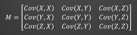
in which, the covariance value between 2 data sets can be computed as:
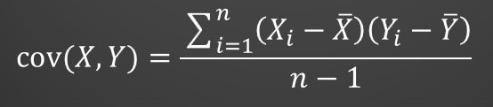
- For the Covariance matrix M, we will find m eigenvectors and m eigenvalues
- Given mxm matrix, we can find m eigenvectors and m eigenvalues
- Eigenvectors can only be found for square matrix.
- Not every square matrix has eigenvectors
- A square matrix A and its transpose have the same eigenvalues but different eigenvectors
- The eigenvalues of a diagonal or triangular matrix are its diagonal elements.
- Eigenvectors of a matrix A with distinct eigenvalues are linearly independent.
Eigenvector with the largest eigenvalue forms the first principal component of the data set … and so on …*
7.2 Implementation
Here we gonna use the breast cancer Wisconsine data set:
from sklearn.datasets import load_breast_cancer
data = load_breast_cancer()
X = data.data
y = data.target

X_train, X_test, y_train, y_test = train_test_split(X,y,train_size=0.6,random_state=123)

X_train_scaled = StandardScaler().fit_transform(X_train)
X_test_scaled = StandardScaler().fit_transform(X_test)
7.2.1 Compute PCA using sklearn:
from sklearn.decomposition import PCA
pca = PCA()
PCs = pca.fit_transform(X_train_scaled)
PCs.shape
We can see that the shape of PCs are [341,30], which has the same 30 inputs/principal components as in the original data
7.2.2 Explained Variance
The explained variance tells you how much information (variance) can be attributed to each of the principal components.
pca.explained_variance_ratio_
print("The first 4 components represent %1.3f" % pca.explained_variance_ratio_[0:4].sum(), " total variance")
Since using only 4 PCs, it is able to represent 30 PCs in the entire data, therefore, we use this 4 PCs to construct the ML model using K-Nearest Neighbors:
7.2.3 Application of PCA model in Machine Learning:
from sklearn.neighbors import KNeighborsClassifier
from sklearn.metrics import accuracy_score as acc_score
pca = PCA(n_components=4) #We choose number of principal components to be 4

X_train_pca = pd.DataFrame(pca.fit_transform(X_train_scaled))
X_test_pca = pd.DataFrame(pca.transform(X_test_scaled))
X_train_pca.columns = ['PC1','PC2','PC3','PC4']
X_test_pca.columns  = ['PC1','PC2','PC3','PC4']

# Use random forest to train model
model_KNN = KNeighborsClassifier().fit(X_train_pca, y_train)
y_pred_KNN = model_KNN.predict(X_test_pca)
print("The accuracy score is %1.3f" % acc_score(y_test,y_pred_KNN))
Plotting the testing result with indicator of Wrong prediction
import matplotlib.pyplot as plt

ax = plt.gca()

targets = np.unique(y_pred_KNN)
colors = ['r', 'g']

for target, color in zip(targets,colors):
    indp = y_pred_KNN == target
    ax.scatter(X_test_pca.loc[indp, 'PC1'], X_test_pca.loc[indp, 'PC2'],c = color)

# Ploting the Wrong Prediction
ind = y_pred_KNN!=np.array(y_test)
ax.scatter(X_test_pca.loc[ind, 'PC1'],X_test_pca.loc[ind, 'PC2'],c = 'black')

#axis control
ax.legend(['malignant','benign','Wrong Prediction'])
ax.set_title("Testing set from KNN using PCA 4 components")
ax.set_xlabel('PC1')
ax.set_ylabel('PC2')

plt.show()
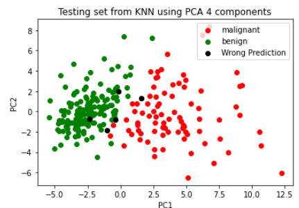
As seen, there are 4 points that were wrongly identified
Key Points
PCA