Training Machine Learning model using Regression Method

Overview

Teaching: 20 min
Exercises: 0 min

Questions

How to train a Machine Learning model using Regression method

Objectives

Learn to use different Regression algorithm for Machine Learning training

5 Supervised Learning training

5.1 For Continuous output

5.1.1 Train model using Linear Regression

Pre-processing data and create partition

library(caret)
data(airquality)

set.seed(123)
#Impute missing value using Bagging approach
PreImputeBag <- preProcess(airquality,method="bagImpute")
airquality_imp <- predict(PreImputeBag,airquality)

indT <- createDataPartition(y=airquality_imp$Ozone,p=0.6,list=FALSE)
training <- airquality_imp[indT,]
testing  <- airquality_imp[-indT,]

Fit a Linear model using method=lm

ModFit <- train(Ozone~Temp,data=training,
                preProcess=c("center","scale"),
                method="lm")
summary(ModFit$finalModel)

Apply trained model to testing data set and evaluate output

prediction <- predict(ModFit,testing)
cor.test(prediction,testing$Ozone)
postResample(prediction,testing$Ozone)

5.1.2 Train model using Multi-Linear Regression

From the above model, the postResample only show the reasonable result:

> postResample(prediction,testing$Ozone)
      RMSE   Rsquared        MAE 
27.6743204  0.4313953 18.5866936 

The reason is that we only build the model with 1 input Temp. In this section, we will build the model with more input Solar Radiation, Wind, Temperature:

modFit2 <- train(Ozone~Solar.R+Wind+Temp,data=training,
                 preProcess=c("center","scale"),
                 method="lm")
summary(modFit2$finalModel)

prediction2 <- predict(modFit2,testing)

cor.test(prediction2,testing$Ozone)
postResample(prediction2,testing$Ozone)

Output is therefore better with smaller RMSE and higher Rsquared:

> postResample(prediction2,testing$Ozone)
      RMSE   Rsquared        MAE 
24.3388752  0.5512334 16.5798881 

5.1.3 Train model using Stepwise Linear Regression

It’s a step by step Regression to determine which covariates set best match with the dependent variable. Using AIC as criteria:

modFit_SLR <- train(Ozone~Solar.R+Wind+Temp,data=training,method="lmStepAIC")
summary(modFit_SLR$finalModel)

prediction_SLR <- predict(modFit_SLR,testing)

cor.test(prediction_SLR,testing$Ozone)
postResample(prediction_SLR,testing$Ozone)

> postResample(prediction_SLR,testing$Ozone)
      RMSE   Rsquared        MAE 
25.0004212  0.5239849 17.0977421 

5.1.4 Train model using Polynomial Regression

In this study, let use polynomial regression with degree of freedom=3

modFit_poly <- train(Ozone~poly(Solar.R,3)+poly(Wind,3)+poly(Temp,3),data=training,
                     preProcess=c("center","scale"),
                     method="lm")
summary(modFit_poly$finalModel)

prediction_poly <- predict(modFit_poly,testing)

cor.test(prediction_poly,testing$Ozone)
postResample(prediction_poly,testing$Ozone)

> postResample(prediction_poly,testing$Ozone)
      RMSE   Rsquared        MAE 
20.8369196  0.6611866 13.7168643 

5.1.5 Train model using Principal Component Regression

Linear Regression using the output of a Principal Component Analysis (PCA). PCR is skillful when data has lots of highly correlated predictors

modFit_PCR <- train(Ozone~Solar.R+Wind+Temp,data=training,method="pcr")
summary(modFit_PCR$finalModel)

prediction_PCR <- predict(modFit_PCR,testing)

cor.test(prediction_PCR,testing$Ozone)
postResample(prediction_PCR,testing$Ozone)

5.2 For categorical output

5.2.1 Train model using Logistic Regression

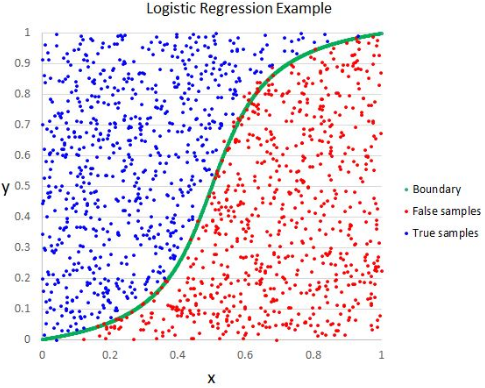
Logistic regression is another technique borrowed by machine learning from the field of statistics. It is the go-to method for binary classification problems (problems with two class values).
Typical binary classification: True/False, Yes/No, Pass/Fail, Spam/No Spam, Male/Female
Unlike linear regression, the prediction for the output is transformed using a non-linear function called the logistic function.
The standard logistic function has formulation:

In this example, we use spam data set from package kernlab. This is a data set collected at Hewlett-Packard Labs, that classifies 4601 e-mails as spam or non-spam. In addition to this class label there are 57 variables indicating the frequency of certain words and characters in the e-mail. More information on this data set can be found here

Train the model:

library(kernlab)
data(spam)
names(spam)

indTrain <- createDataPartition(y=spam$type,p=0.6,list = FALSE)
training <- spam[indTrain,]
testing  <- spam[-indTrain,]

ModFit_glm <- train(type~.,data=training,method="glm")
summary(ModFit_glm$finalModel)

Predict based on testing data and evaluate model output:

predictions <- predict(ModFit_glm,testing)
confusionMatrix(predictions, testing$type)

Plotting ROC and computing AUC:

#Need to install package ROCR
library(ROCR)
pred_prob <- predict(ModFit_glm,testing, type = "prob")
head(pred_prob)
data_roc <- data.frame(pred_prob = pred_prob[,'spam'],
                           actual_label = ifelse(testing$type == 'spam', 1, 0))

roc <- prediction(predictions = data_roc$pred_prob,
                      labels = data_roc$actual_label)

plot(performance(roc, "tpr", "fpr"))
abline(0, 1, lty = 2)
auc <- performance(roc, measure = "auc")
auc@y.values

Key Points

Regression training

previous episode

Introduction to Machine Learning using R

next episode