Dimension Reduction
Overview
Teaching: 20 min
Exercises: 0 minQuestions
What happen when there are lots of covariates?
Objectives
Learn how to apply PCA in ML model
10 Principal Component Analysis
- Handy with large data
- Where many variables correlate with one another, they will all contribute strongly to the same principal component
- Each principal component sums up a certain percentage of the total variation in the dataset
- More Principal Components, more summarization of the original data sets
10.1 Explanation
- For example, we have 3 data sets:
X, Y, Z - We need to compute the covariance matrix M for the 3 data set:

in which, the covariance value between 2 data sets can be computed as:

- For the Covariance matrix M, we will find m eigenvectors and m eigenvalues
- Given mxm matrix, we can find m eigenvectors and m eigenvalues
- Eigenvectors can only be found for square matrix.
- Not every square matrix has eigenvectors
- A square matrix A and its transpose have the same eigenvalues but different eigenvectors
- The eigenvalues of a diagonal or triangular matrix are its diagonal elements.
- Eigenvectors of a matrix A with distinct eigenvalues are linearly independent.
Eigenvector with the largest eigenvalue forms the first principal component of the data set … and so on …*
10.2 Implementation
10.2.1 Compute PCA using eigenvector:
library(PerformanceAnalytics)
data(mtcars)
#Ignore vs & am (PCA works good with numeric data )
datain <- mtcars[,c(1:7,10:11)]
chart.Correlation(datain)
cin <- cov(scale(datain))
ein <- eigen(cin)
newpca <-   -scale(datain) %*% ein$vectors
10.2.2 Compute PCA using built-in function:
mtcars.pca <- prcomp(datain,center=TRUE,scale=TRUE)
summary(mtcars.pca)
10.2.3 A nice way to plot PCA:
Install ggbiplot package:
library(devtools)
install_github("vqv/ggbiplot")
library(ggbiplot)
ggbiplot(mtcars.pca)
ggbiplot(mtcars.pca, labels=rownames(mtcars))
ggbiplot(mtcars.pca,ellipse=TRUE,  labels=rownames(mtcars))

mtcars.country <- c(rep("Japan", 3), rep("US",4), rep("Europe", 7),rep("US",3), "Europe", rep("Japan", 3), rep("US",4), rep("Europe", 3), "US", rep("Europe", 3))

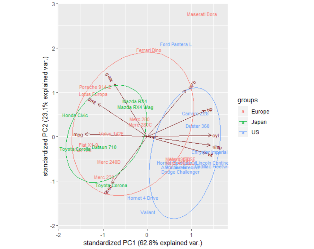
ggbiplot(mtcars.pca,ellipse=TRUE,labels=rownames(mtcars),groups = mtcars.country)
10.2.4 Application of PCA model in Machine Learning:
data(mtcars)
set.seed(123)
datain <- mtcars[,c(1:7,10:11)]

indT <- createDataPartition(y=datain$mpg,p=0.6,list=FALSE)
training <- datain[indT,]
testing  <- datain[-indT,]

preProc <- preProcess(training[,-1],method="pca",pcaComp = 1)
trainPC <- predict(preProc,training[,-1])
testPC  <- predict(preProc,testing[,-1])

traindat<- cbind(training$mpg,trainPC)
testdat <- cbind(testing$mpg,testPC)

names(traindat) <- c("mpg","PC1")
names(testdat)  <- names(traindat)

modFitPC<- train(mpg~.,method="lm",data=traindat)

predictand <- predict(modFitPC,testdat)
postResample(testing$mpg,as.vector(predictand))
Key Points
PCA