Introduction to Machine Learning

Overview

Teaching: 10 min
Exercises: 0 min

Questions

What is Machine Learning

Objectives

Learng basic about Machine Learning

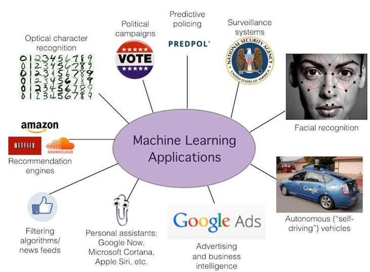
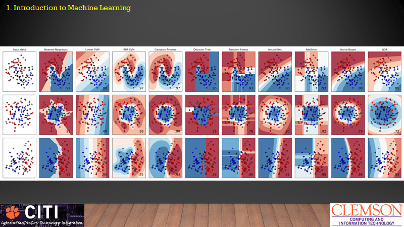
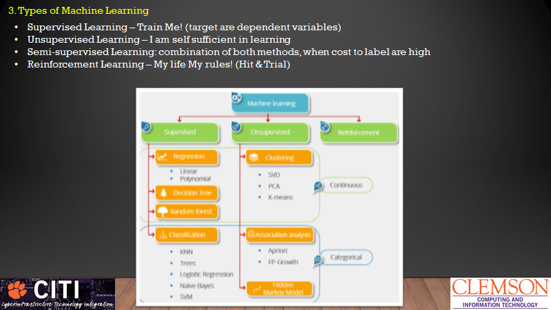
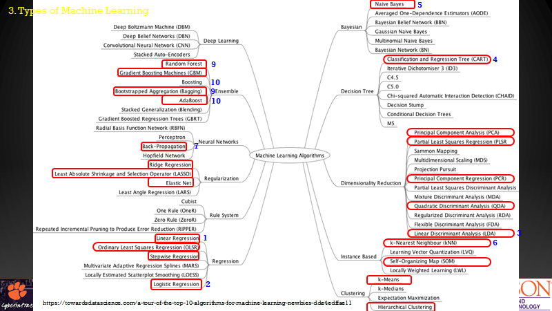
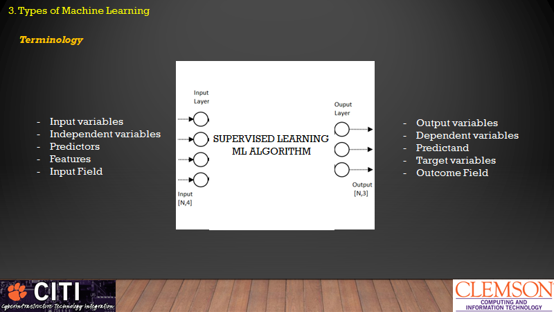
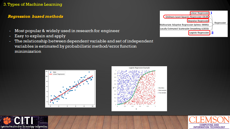
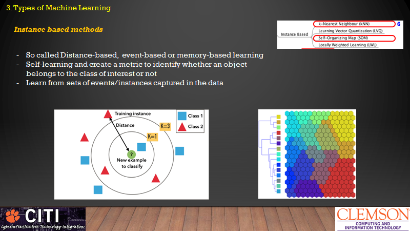
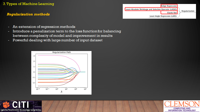
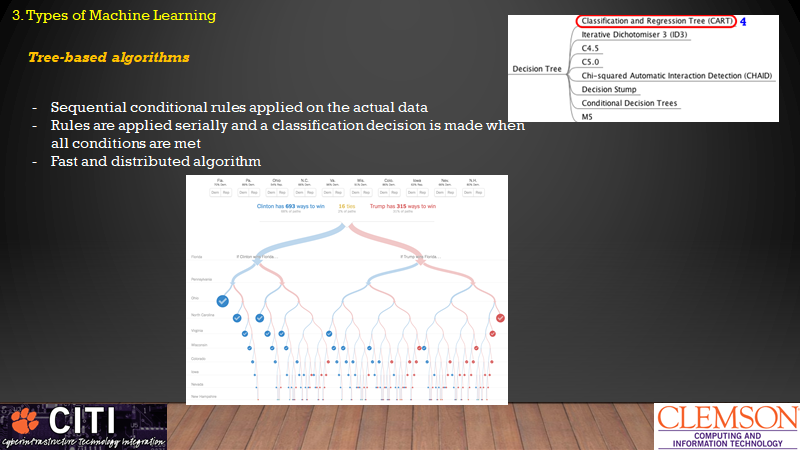
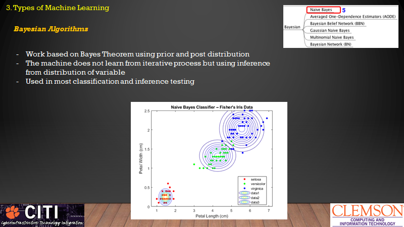
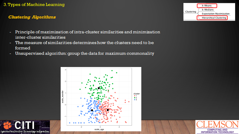
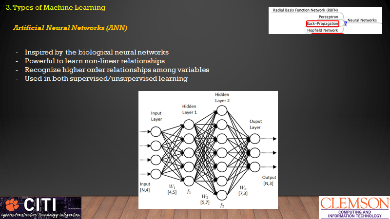
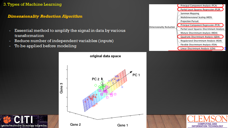
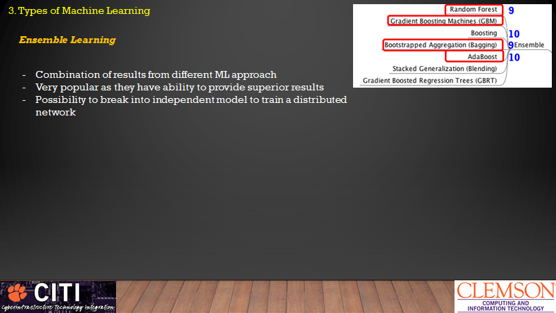
Supervised Learning model that we are going to learn:

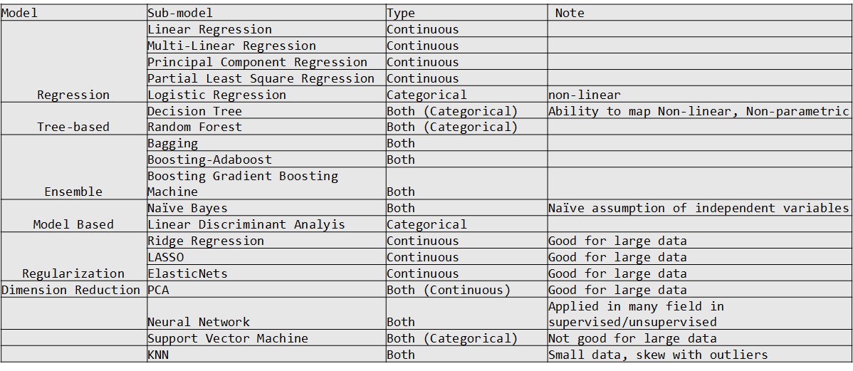
Key Points

Basic Machine Learning

Introduction to Caret

Overview

Teaching: 40 min
Exercises: 0 min

Questions

What is Caret

Objectives

Master Caret package for Machine Learning

2.1 What is Caret

The caret package (short for Classification And REgression Training) is a set of functions that attempt to streamline the process for creating predictive models. The package contains tools for:

data splitting pre-processing feature selection model tuning using resampling variable importance estimation as well as other functionality.

There are many different modeling functions in R. Some have different syntax for model training and/or prediction. The package started off as a way to provide a uniform interface the functions themselves, as well as a way to standardize common tasks (such parameter tuning and variable importance).

The current release version can be found on CRAN and the project is hosted on github. Caret was developed by Max Kuhn Here only touch some of the very basic command that is useful for our Machine Learning class.

caret cheatsheet

2.2 Why using Caret

R has so many ML algorithms, challenge to keep track, different syntax for different packages
Possibly the biggest project in R
All in one supervised learning problem
Uniform interface
Standard pre & post processing

2.3 Install `caret`

In R console:

install.packages("caret", dependencies = c("Depends", "Suggests"))

In R studio:

Select Tools\Install Packages and select caret from CRAN

Once installed, load the caret package to make sure that it works:

library(caret)

2.4 Pre-processing using `caret`

There are several steps that we will use caret for. For preprocessing raw data, we gonna use caret in these tasks:

Preprocessing with missing value
Data partition: training and testing

2.4.1 Visualize important variables

Here we introduce the library GGally with function ggpairs to help user in visualizing the input data

library(GGally)
ggpairs(data=iris,aes(colour=Species))

2.4.2 Pre-processing with missing value

Most of the time the input data has missing values (NA, NaN, Inf) due to data collection issue (power, sensor, personel).
There are three main problems that missing data causes: missing data can introduce a substantial amount of bias, make the handling and analysis of the data more arduous, and create reductions in efficiency
These missing values need to be treated/cleaned before we can use because “Garbage in => Garbage out”.
There are several ways to treat the missing values:

Method 1: remove all missing NA values

data("airquality") # Here we use this sample data because it contains missing value
new_airquality1 <- na.omit(airquality)

Method 2: Set NA to mean value

NA2mean <- function(x) replace(x, is.na(x), mean(x, na.rm = TRUE))
new_airquality2 <-replace(airquality, TRUE, lapply(airquality, NA2mean))

Method 3: Use Impute to handle missing values In statistics, imputation is the process of replacing missing data with substituted values. Because missing data can create problems for analyzing data, imputation is seen as a way to avoid pitfalls involved with listwise deletion of cases that have missing values. That is to say, when one or more values are missing for a case, most statistical packages default to discarding any case that has a missing value, which may introduce bias or affect the representativeness of the results. Imputation preserves all cases by replacing missing data with an estimated value based on other available information. Once all missing values have been imputed, the data set can then be analysed using standard techniques for complete data. There have been many theories embraced by scientists to account for missing data but the majority of them introduce bias. A few of the well known attempts to deal with missing data include: hot deck and cold deck imputation; listwise and pairwise deletion; mean imputation; non-negative matrix factorization; regression imputation; last observation carried forward; stochastic imputation; and multiple imputation.

Here we use preProcess function from caret to perform bagImpute (Bootstrap Aggregation Imputation):

library(caret)
PreImputeBag <- preProcess(airquality,method="bagImpute")
DataImputeBag <- predict(PreImputeBag,airquality)

In addition to bagImpute, we also can use knnImpute (K-Nearest Neighbour Imputation) knnImpute can also be used to impute missing value, however, it standardize the data after Imputing:

MData <- airquality[,-c(1,5,6)]
PreImputeKNN <- preProcess(MData,method="knnImpute",k=5)
DataImputeKNN <- predict(PreImputeKNN,MData)

#Convert back to original scale
RescaleDataM <- t(t(DataImputeKNN)*PreImputeKNN$std+PreImputeKNN$mean)

Note bagImpute is more powerful and computational cost than knnImpute

Key Points

Caret

Data Partition with caret

Overview

Teaching: 20 min
Exercises: 0 min

Questions

What is Data Partition

Objectives

Learn how to split data using caret

3 Data partition: training and testing

In Machine Learning, it is mandatory to have training and testing set. Some time a verification set is also recommended. Here are some functions for spliting training/testing set in caret:
createDataPartition: create series of test/training partitions
createResample creates one or more bootstrap samples.
createFolds splits the data into k groups
createTimeSlices creates cross-validation split for series data.
groupKFold splits the data based on a grouping factor.

Due to time constraint, we only focus on createDataPartition and createFolds

3.1 Data spliting using `Data Partition`

Here we use createDataPartition to randomly split 60% data for training and the rest for testing:

ind1 <- createDataPartition(y=iris$Species,p=0.6,list=FALSE,times=1)
#list=FALSE, prevent returning result as a list
#times=1 to create the resample size. Default value is 1.
training <- iris[ind1,]
testing  <- iris[-ind1,] 

3.2 Data spliting using `K-fold`: Cross validation approach

The procedure has a single parameter called k that refers to the number of groups that a given data sample is to be split into. As such, the procedure is often called k-fold cross-validation. When a specific value for k is chosen, it may be used in place of k in the reference to the model, such as k=10 becoming 10-fold cross-validation.

fitControl <- trainControl(method="cv", number=10)
# train the model
model <- train(Species~., data=training, 
               trControl=fitControl, method="lda")
# summarize results
print(model)
predict1 <- predict(model,testing)

3.3 Other Cross-Validation approach

method: The resampling method: “boot”, “cv”, “LOOCV”, “LGOCV”, “repeatedcv”, “timeslice”, “none” and “oob”

More information on model tuning using caret can be found here

Key Points

Caret

Evaluation Metrics with caret

Overview

Teaching: 40 min
Exercises: 0 min

Questions

How do we measure the accuracy of ML model

Objectives

Learn different metrics with caret

4 Evaluation Metrics

Evaluation Metric is an essential part in any Machine Learning project.
It measures how good or bad is your Machine Learning model
Different Evaluation Metrics are used for Regression model (Continuous output) or Classification model (Categorical output).

4.1 Regression model Evaluation Metrics

4.1.1 Correlation Coefficient (R) or Coefficient of Determination (R2):

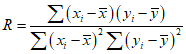
cor(prediction,testing)
cor.test(prediction,testing)

4.1.2 Root Mean Square Error (RMSE) or Mean Square Error (MSE)

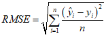
The postResample function gives RMSE, R2 and MAE at the same time:

postResample(prediction,testing$Ozone)

4.2. Classification model Evaluation Metrics

4.2.1 Confusion Matrix

A confusion matrix is a technique for summarizing the performance of a classification algorithm.
You can learn more about Confusion Matrix here

For binary output (classification problem with only 2 output type, also most popular):

 confusionMatrix(predict,testing)

Key Points

Caret

Training Machine Learning model using Regression Method

Overview

Teaching: 20 min
Exercises: 0 min

Questions

How to train a Machine Learning model using Regression method

Objectives

Learn to use different Regression algorithm for Machine Learning training

5 Supervised Learning training

5.1 For Continuous output

5.1.1 Train model using Linear Regression

Pre-processing data and create partition

library(caret)
data(airquality)

set.seed(123)
#Impute missing value using Bagging approach
PreImputeBag <- preProcess(airquality,method="bagImpute")
airquality_imp <- predict(PreImputeBag,airquality)

indT <- createDataPartition(y=airquality_imp$Ozone,p=0.6,list=FALSE)
training <- airquality_imp[indT,]
testing  <- airquality_imp[-indT,]

Fit a Linear model using method=lm

ModFit <- train(Ozone~Temp,data=training,
                preProcess=c("center","scale"),
                method="lm")
summary(ModFit$finalModel)

Apply trained model to testing data set and evaluate output

prediction <- predict(ModFit,testing)
cor.test(prediction,testing$Ozone)
postResample(prediction,testing$Ozone)

5.1.2 Train model using Multi-Linear Regression

From the above model, the postResample only show the reasonable result:

> postResample(prediction,testing$Ozone)
      RMSE   Rsquared        MAE 
27.6743204  0.4313953 18.5866936 

The reason is that we only build the model with 1 input Temp. In this section, we will build the model with more input Solar Radiation, Wind, Temperature:

modFit2 <- train(Ozone~Solar.R+Wind+Temp,data=training,
                 preProcess=c("center","scale"),
                 method="lm")
summary(modFit2$finalModel)

prediction2 <- predict(modFit2,testing)

cor.test(prediction2,testing$Ozone)
postResample(prediction2,testing$Ozone)

Output is therefore better with smaller RMSE and higher Rsquared:

> postResample(prediction2,testing$Ozone)
      RMSE   Rsquared        MAE 
24.3388752  0.5512334 16.5798881 

5.1.3 Train model using Stepwise Linear Regression

It’s a step by step Regression to determine which covariates set best match with the dependent variable. Using AIC as criteria:

modFit_SLR <- train(Ozone~Solar.R+Wind+Temp,data=training,method="lmStepAIC")
summary(modFit_SLR$finalModel)

prediction_SLR <- predict(modFit_SLR,testing)

cor.test(prediction_SLR,testing$Ozone)
postResample(prediction_SLR,testing$Ozone)

> postResample(prediction_SLR,testing$Ozone)
      RMSE   Rsquared        MAE 
25.0004212  0.5239849 17.0977421 

5.1.4 Train model using Polynomial Regression

In this study, let use polynomial regression with degree of freedom=3

modFit_poly <- train(Ozone~poly(Solar.R,3)+poly(Wind,3)+poly(Temp,3),data=training,
                     preProcess=c("center","scale"),
                     method="lm")
summary(modFit_poly$finalModel)

prediction_poly <- predict(modFit_poly,testing)

cor.test(prediction_poly,testing$Ozone)
postResample(prediction_poly,testing$Ozone)

> postResample(prediction_poly,testing$Ozone)
      RMSE   Rsquared        MAE 
20.8369196  0.6611866 13.7168643 

5.1.5 Train model using Principal Component Regression

Linear Regression using the output of a Principal Component Analysis (PCA). PCR is skillful when data has lots of highly correlated predictors

modFit_PCR <- train(Ozone~Solar.R+Wind+Temp,data=training,method="pcr")
summary(modFit_PCR$finalModel)

prediction_PCR <- predict(modFit_PCR,testing)

cor.test(prediction_PCR,testing$Ozone)
postResample(prediction_PCR,testing$Ozone)

5.2 For categorical output

5.2.1 Train model using Logistic Regression

Logistic regression is another technique borrowed by machine learning from the field of statistics. It is the go-to method for binary classification problems (problems with two class values).
Typical binary classification: True/False, Yes/No, Pass/Fail, Spam/No Spam, Male/Female
Unlike linear regression, the prediction for the output is transformed using a non-linear function called the logistic function.
The standard logistic function has formulation:

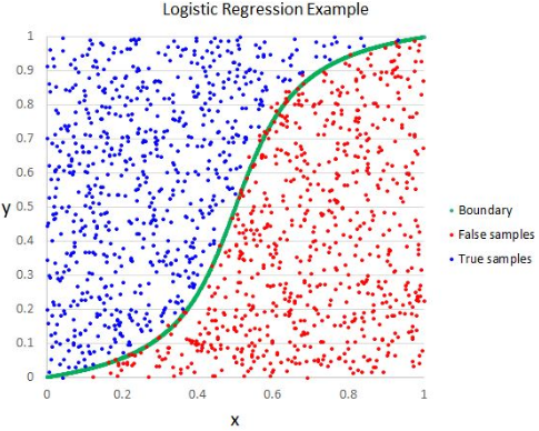
In this example, we use spam data set from package kernlab. This is a data set collected at Hewlett-Packard Labs, that classifies 4601 e-mails as spam or non-spam. In addition to this class label there are 57 variables indicating the frequency of certain words and characters in the e-mail. More information on this data set can be found here

Train the model:

library(kernlab)
data(spam)
names(spam)

indTrain <- createDataPartition(y=spam$type,p=0.6,list = FALSE)
training <- spam[indTrain,]
testing  <- spam[-indTrain,]

ModFit_glm <- train(type~.,data=training,method="glm")
summary(ModFit_glm$finalModel)

Predict based on testing data and evaluate model output:

predictions <- predict(ModFit_glm,testing)
confusionMatrix(predictions, testing$type)

Plotting ROC and computing AUC:

#Need to install package ROCR
library(ROCR)
pred_prob <- predict(ModFit_glm,testing, type = "prob")
head(pred_prob)
data_roc <- data.frame(pred_prob = pred_prob[,'spam'],
                           actual_label = ifelse(testing$type == 'spam', 1, 0))

roc <- prediction(predictions = data_roc$pred_prob,
                      labels = data_roc$actual_label)

plot(performance(roc, "tpr", "fpr"))
abline(0, 1, lty = 2)
auc <- performance(roc, measure = "auc")
auc@y.values

Key Points

Regression training

Training Machine Learning model using Tree-based model

Overview

Teaching: 20 min
Exercises: 0 min

Questions

How to train a Machine Learning model using Tree-based model

Objectives

Learn to use different Tree-based algorithm for Machine Learning training

Supervised Learning training

Train model using Decision Tree

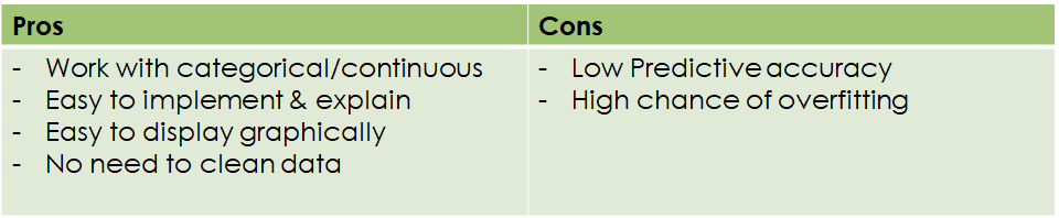
Tree based learning algorithms are considered to be one of the best and mostly used supervised learning methods.
Tree based methods empower predictive models with high accuracy, stability and ease of interpretation
Non-parametric and non-linear relationships
Types: Categorical and Continuous

Spliting algorithm

Gini Impurity: (Categorical)
Chi-Square index (Categorical)
Cross-Entropy & Information gain (Categorical)
Reduction Variance (Continuous)

Pros & Cons

Implementation

Here we will use iris data

library(caret)
data(iris)
set.seed(123)
indT <- createDataPartition(y=iris$Species,p=0.6,list=FALSE)
training <- iris[indT,]
testing  <- iris[-indT,]

Next we will train using method="rpart" with gini splitting algorithm:

ModFit_rpart <- train(Species~.,data=training,method="rpart",
                      parms = list(split = "gini"))
# gini can be replaced by chisquare, entropy, information

#fancier plot
library(rattle)
fancyRpartPlot(ModFit_rpart$finalModel)

Apply decision tree model to predict output of testing data

predict_rpart <- predict(ModFit_rpart,testing)
confusionMatrix(predict_rpart, testing$Species)

testing$PredRight <- predict_rpart==testing$Species
ggplot(testing,aes(x=Petal.Width,y=Petal.Length))+
  geom_point(aes(col=PredRight))

Train model using Random Forest

Random Forest is considered to be a panacea of all data science problems. On a funny note, when you can’t think of any algorithm (irrespective of situation), use random forest!
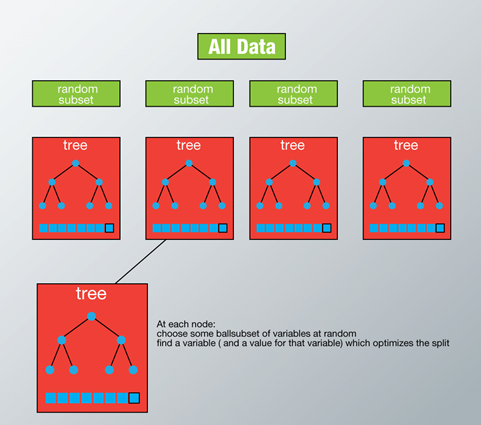
Opposite to Decision Tree, Random Forest use bootstrapping technique to grow multiple tree
Random Forest is a versatile machine learning method capable of performing both regression and classification tasks.
It is a type of ensemble learning method, where a group of weak models combine to form a powerful model.
The end output of the model is like a black box and hence should be used judiciously.
Detail explaination
If there are M input variables, a number m<M is specified such that at each node, m variables are selected at random out of the M. The best split on these m is used to split the node. The value of m is held constant while we grow the forest.
Each tree is grown to the largest extent possible and there is no pruning.
Predict new data by aggregating the predictions of the ntree trees (i.e., majority votes for classification, average for regression).

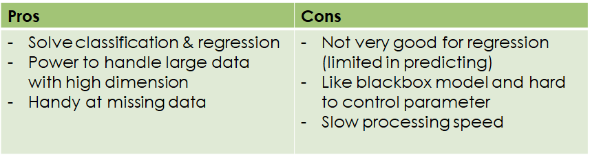
Pros & Cons of Random Forest

Implementation of Random Forest

ModFit_rf <- train(Species~.,data=training,method="rf",prox=TRUE)

predict_rf <- predict(ModFit_rf,testing)
confusionMatrix(predict_rf, testing$Species)

testing$PredRight <- predict_rf==testing$Species
ggplot(testing,aes(x=Petal.Width,y=Petal.Length))+
  geom_point(aes(col=PredRight))

We can see that Random Forest result has better prediction than Decision Tree

Key Points

Decision Tree, Random Forest

Training Machine Learning model using Ensemble approach

Overview

Teaching: 20 min
Exercises: 0 min

Questions

How to overcome limitation of single ML model?

Objectives

Learn to use different Ensemble ML algorithm for Machine Learning training

7.1 Why Ensemble:

Ensemble is a method in Machine Learning that combine decision from several ML models to obtain optimum output. This espisode get information from here

Source: Patheos.com

Ensemble approaches can reduce variance & Avoid Overfitting by combining results of multiple classifiers on different sub-samples

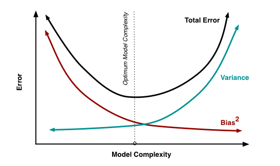
7.2 Train model using Ensemble Approach

Ensemble methods use multiple learning algorithms to obtain better predictive performance than could be obtained from any of the constituent learning algorithms alone. Unlike a statistical ensemble in statistical mechanics, which is usually infinite, a machine learning ensemble consists of only a concrete finite set of alternative models, but typically allows for much more flexible structure to exist among those alternatives. Here we will be learning several ensemble models:

Random Forest
Bagging
Boosting with AdaBoost
Boosting with Gradient Boosting Machine

7.3 Train model using Bagging (Bootstrap Aggregation)

The bootstrap method is a resampling technique used to estimate statistics on a population by sampling a dataset with replacement.
Bootstrap randomly create a small subsets of data from entire dataset
The subset data has similar characteristic as the entire dataset.

7.3.1 Detail explaination of Bagging

There are 3 steps in Bagging

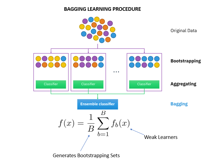
Step 1: Here you replace the original data with new sub-sample data using bootstrapping.

Step 2: Train each sub-sample data using ML algorithm

Step 3: Lastly, you use an average value to combine the predictions of all the classifiers, depending on the problem. Generally, these combined values are more robust than a single model.

Bagging in R can be used in many different model:

ctreebag: used for Decision Tree
bagFDA: used for Flexible Discriminant Analysis
ldaBag: Bagging for Linear Discriminant Analysis
plsBag: Bagging for Principal Linear Regression

7.3.2 Implementation of Bagging using decision Tree

ModFit_bag <- train(as.factor(Species) ~ .,data=training,
                   method="treebag",
                   importance=TRUE)
predict_bag <- predict(ModFit_bag,testing)
confusionMatrix(predict_bag, testing$Species)
plot(varImp(ModFit_bag))

7.4 Train model using Boosting

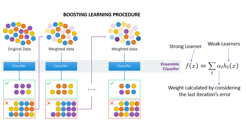
Boosting is an approach to convert weak predictors to get stronger predictors.
Boosting follows a sequential order: output of base learner will be input to another
If a base classifier is misclassifier (red box), its weight is increased and the next base learner will classify more correctly.
Finally combine the classifier to predict result

7.4.1 Adaptive Boosting: Adaboost

Adaptive: weaker learners are tweaked by misclassify from previous classifier
AdaBoost is best used to boost the performance of decision trees on binary classification problems.
Better for classification rather than regression.
Sensitive to noise

In the following example, we use the package adabag, not from caret

library(adabag)

ModFit_adaboost <- boosting(Species~.,data=training,mfinal = 10, coeflearn = "Breiman")
importanceplot(ModFit_adaboost)
predict_Ada <- predict(ModFit_adaboost,newdata=testing)
confusionMatrix(testing$Species,as.factor(predict_Ada$class))

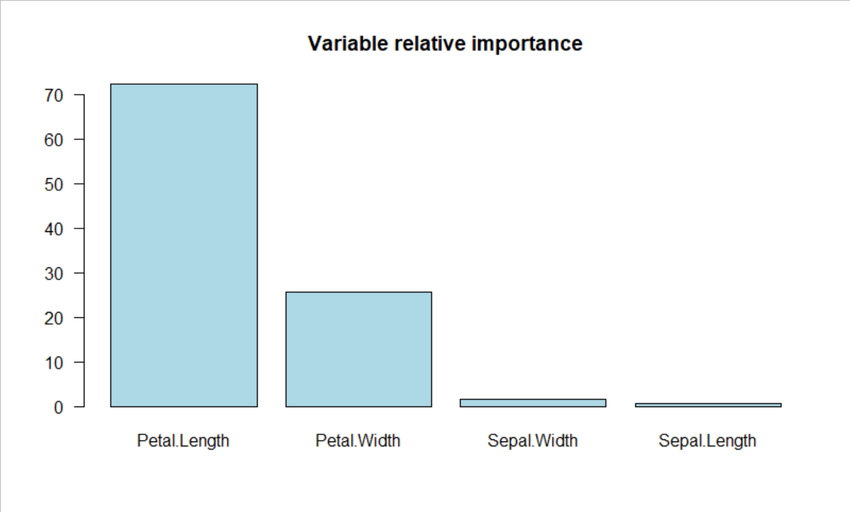
You can see the weight of different predictors from boosting model

7.4.2 Gradient Boosting Machines:

Extremely popular ML algorithm
Widely used in Kaggle competition
Ensemble of shallow and weak successive tree, with each tree learning and improving on the previous

ModFit_GBM <- train(Species~.,data=training,method="gbm",verbose=FALSE)
ModFit_GBM$finalModel
predict_GBM <- predict(ModFit_GBM,newdata=testing)
confusionMatrix(testing$Species,predict_GBM)

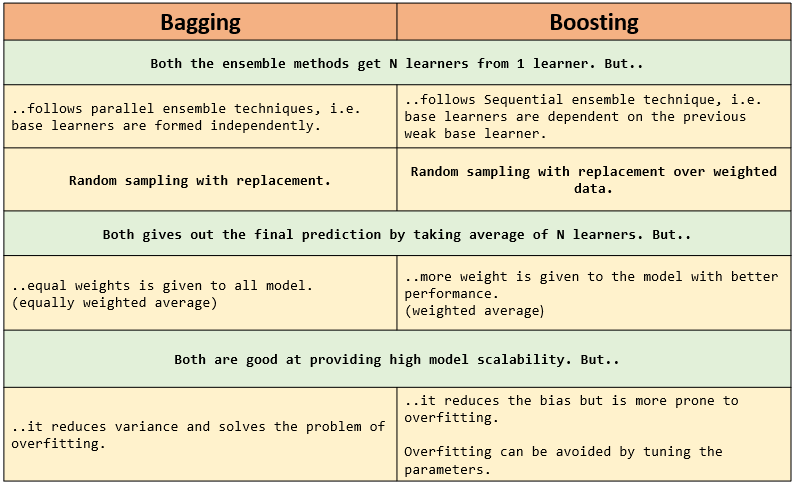
7.5 Compare Bagging and Boosting technique:

7.6 Conclusions

Ensemble overcome the limitation of using only single model
Between bagging and boosting, there is no better approach without trial & error.

Key Points

Bagging, Boosting

Training Machine Learning model using Model based Prediction

Overview

Teaching: 20 min
Exercises: 0 min

Questions

What is model based prediction algorithm in ML?

Objectives

Learn to use different Model based prediction for Machine Learning training

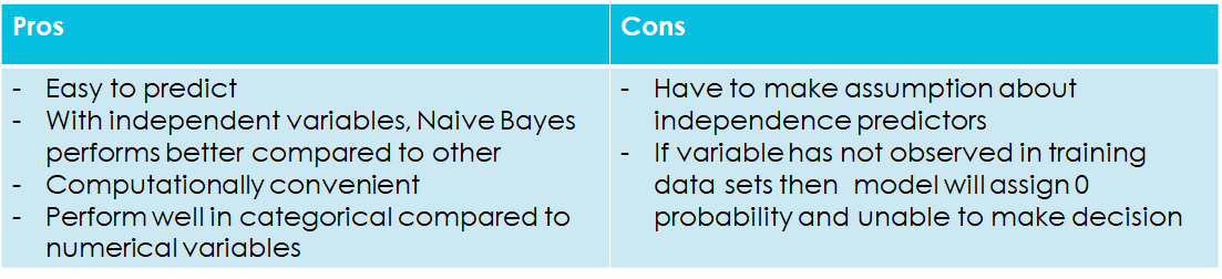
8.1 Naive Bayes

Assuming data follow a probabilistic model
Assuming all predictors are independent (Naïve assumption)
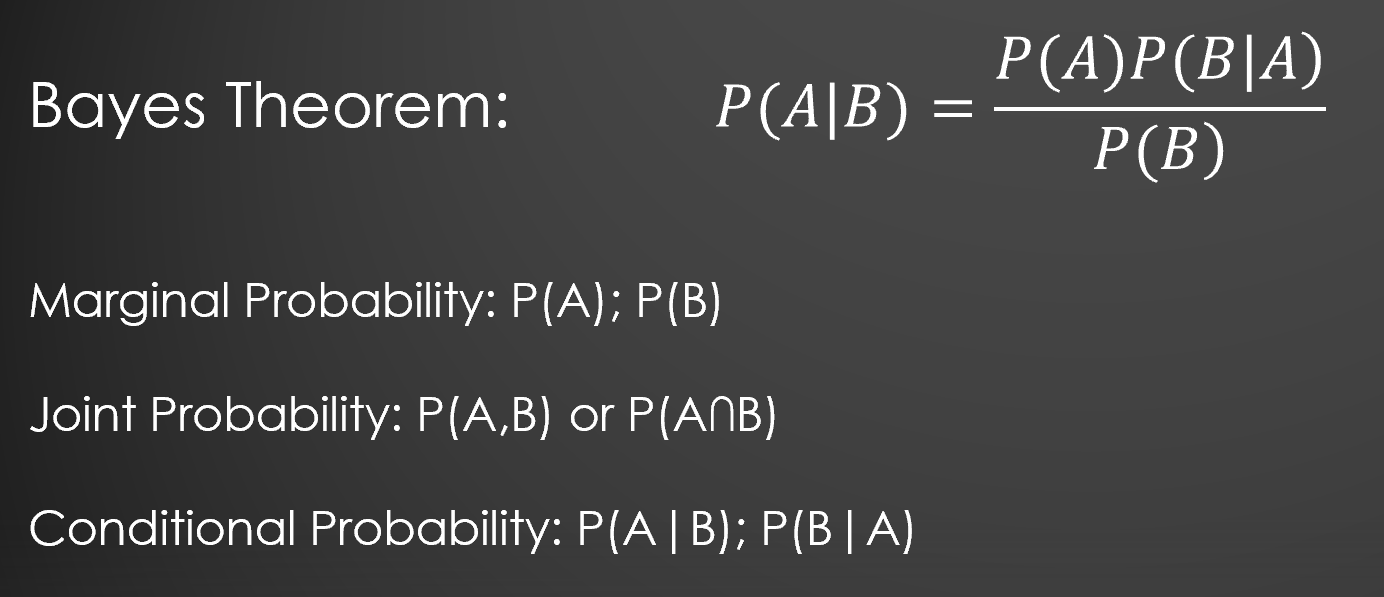
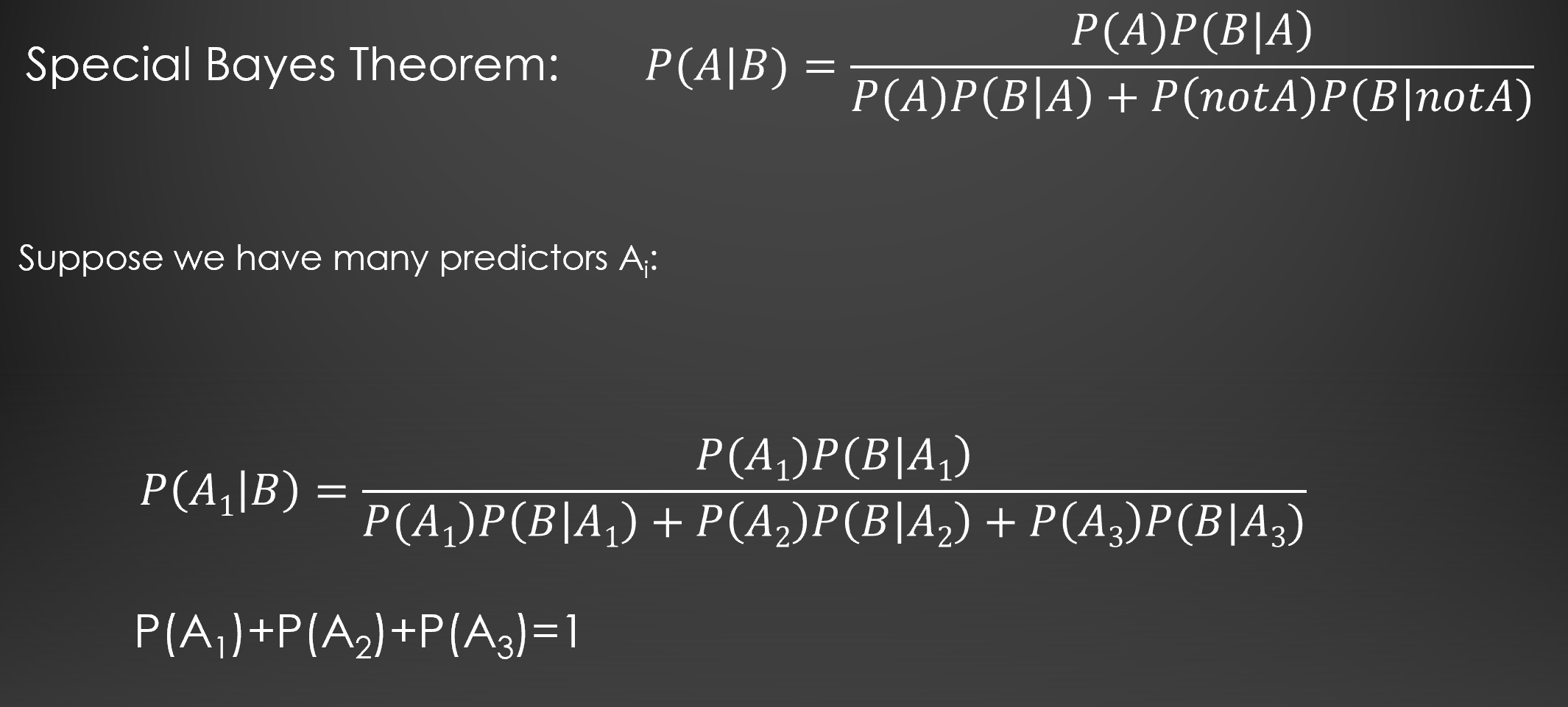
Use Bayes’s theorem to identify optimal classifiers

8.1 Implementation Naive Bayes

ModFit_NB <- train(Species~., data=training, method="nb")

predict_NB <- predict(ModFit_NB,testing)
confusionMatrix(testing$Species,predict_NB)

8.2 Linear Discriminent Analysis

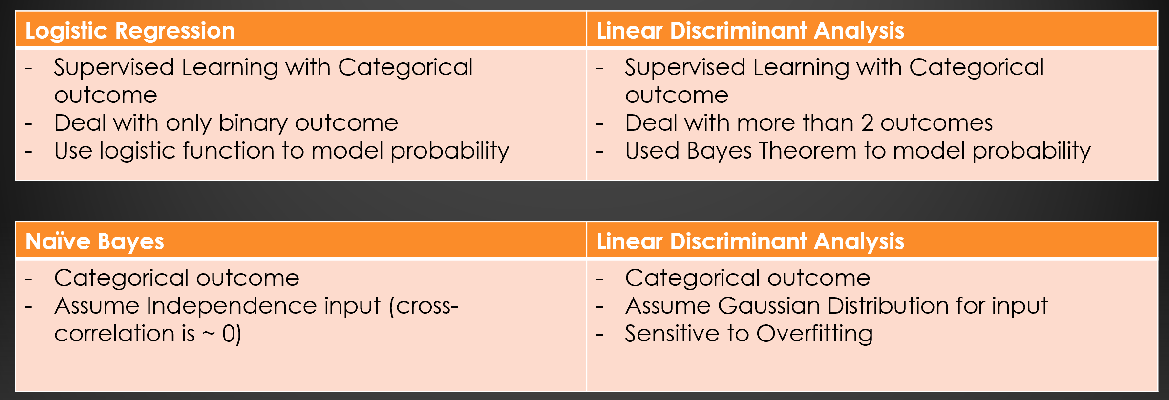
LDA is a supervised learning model that is similar to logistic regression in that the outcome variable is categorical and can therefore be used for classification.
LDA is useful with two or more class of objects

8.2.1 Implementation LDA

ModFit_LDA <- train(Species~., data=training, method="lda")

predict_LDA <- predict(ModFit_LDA,testing)
confusionMatrix(testing$Species,predict_LDA)

Ensemble approach (Bagging) with LDA

ModFit_ldabag <- train(training[,-5],training$Species,method="bag",B=500,
                       bagControl=bagControl(fit=ldaBag$fit,
                                             predict=ldaBag$pred,
                                             aggregate = ldaBag$aggregate))

predict_bag <- predict(ModFit_ldabag,testing)
confusionMatrix(predict_bag, testing$Species)

Key Points

Naive Bayes, Linear Discriminent Analyst

Regularization and Variable Selection

Overview

Teaching: 20 min
Exercises: 0 min

Questions

Why do we need Regularization and Variable Selection in ML model

Objectives

Learn how to apply Regularization and Variable selection in ML model

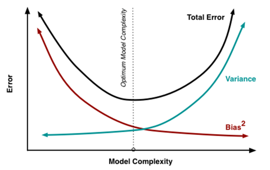
One of the major aspects of training your machine learning model is to avoid overfitting (Using more parameter to best fit the training but on the other hand, failed to evaluate the testing).
The concept of balancing bias and variance, is helpful in understanding the phenomenon of overfitting

9 Regularization

In order to reduce the Model Complexity or to avoid Multi-Collinearity, one needs to reduce the number of covariates (or set the coefficient to be zero).
If the coefficients are too large, let’s penalize them to enforce them to be smaller
Regularization is a form of multilinear regression, that constrains/regularizes or shrinks the coefficient estimates towards zero.
In other words, this technique discourages learning a more complex or flexible model, so as to avoid the risk of overfitting
A simple Multi-Linear Regression look like this:

=> in which: β represents the coefficient estimates for different variables or predictors(x)

The residual sum of squares RSS is the loss function of the fitting procedure. And we need to determine the optimal coefficients 𝛽 to minimize the loss function

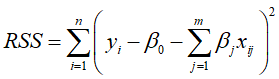
This procedure will adjust the β based on the training data. If there is any noise in training data, the model will not perform well for testing data. Thus, Regularization comes in and regularizes/shrinkage these 𝛽 towards zero.

There are 3 main types of Regularization.

Ridge Regression
LASSO
Elastics Nets

9.1 Ridge Regression

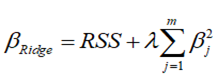
𝜆: Regularization Penalty, to be selected that the model minimized the error

The Ridge Regression loss function contains 2 elements: (1) RSS is actually the Ordinary Least Square (OLS) function for MLR and (2) The regularization term with 𝜆:

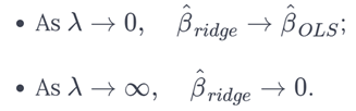
Selecting good 𝜆 is essential. In this case, Cross Validation method should be used
Ridge Regression enforces β to be lower but not 0. By doing so, it will not get rid of irrelevant features but rather minimize their impact on the trained model.
In statistics the coefficient esimated produced by this method is know as L2 norm
It is good practice to normalize predictors to the same sacle before performing Ridge Regression (Because in OLS, the coefficients are scale equivalent)

9.1.2 Implementation

Setting up training/testing model:

library(caret)
#library(ElemStatLearn)=> available for R package > 3.6.2
prostate=read.csv("https://raw.githubusercontent.com/vuminhtue/Machine-Learning-Python/master/data/prostate_data.csv")


set.seed(123)
indT <- which(prostate$train==TRUE)
training <- prostate[indT,]
testing  <- prostate[-indT,]

library(PerformanceAnalytics)
chart.Correlation(training[,-10])

Predict using Ridge Regression method:

library(glmnet)
library(plotmo)
y <- training$lpsa
x <- training[,-c(9,10)]
x <- as.matrix(x)

cvfit_Ridge    <- cv.glmnet(x,y,alpha=0)
plot(cvfit_Ridge)

log(cvfit_Ridge$lambda.min)
log(cvfit_Ridge$lambda.1se)
coef(cvfit_Ridge,s=cvfit_Ridge$lambda.1se)

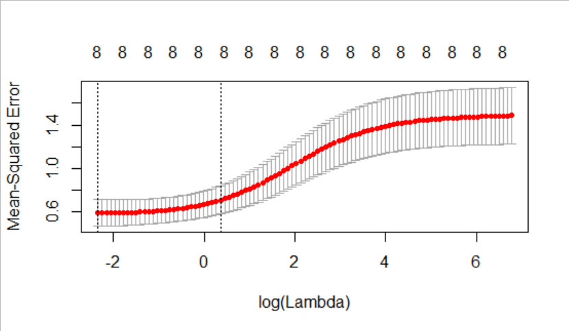
The plot shows the Mean Square Error based on training model with 𝜆 variation.
Top of the chart shows number of predictors used.
There are 2 𝜆 values: (1) 𝜆.min which can be computed using log(cvfit_Ridge$lambda.min) and (2) 𝜆.1se (1 standard error from min value) which can be computed using log(cvfit_Ridge$lambda.1se)
The β values for each predictors can be found using coef(cvfit_Ridge,s=cvfit_Ridge$lambda.1se) or coef(cvfit_Ridge,s=cvfit_Ridge$lambda.min)

Fit_Ridge <- glmnet(x,y,alpha=0,standardize = TRUE)
plot_glmnet(Fit_Ridge,label=TRUE,xvar="lambda",
            col=seq(1,8),grid.col = 'lightgray')

xtest <- testing[,-c(9,10)]
xtest <- as.matrix(xtest)

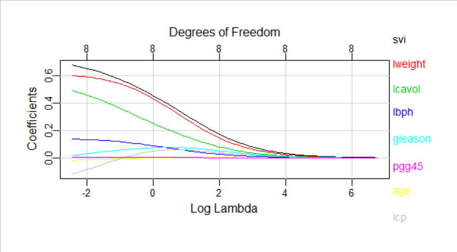
The plot shows different coefficients for all predictors with 𝜆 variation. Using 𝜆.1se, we obtain reasonable result.

> predict_Ridge <- predict(cvfit_Ridge,newx=xtest,s="lambda.1se")
> cor.test(predict_Ridge,testing$lpsa)

	Pearson's product-moment correlation

data:  predict_Ridge and testing$lpsa
t = 5.5527, df = 28, p-value = 6.138e-06
alternative hypothesis: true correlation is not equal to 0
95 percent confidence interval:
 0.4919694 0.8599222
sample estimates:
      cor 
0.7239285 

> postResample(predict_Ridge,testing$lpsa)
     RMSE  Rsquared       MAE 
0.7365551 0.5240725 0.5499648

Ridge Regression’s pros: the pros of RR method over OLS is rooted in the bias variance trade-off. As when 𝜆 increases, the flexibility of RR fit decreases, hence decrease the variance but increase the bias
Ridge Regression’s cons: β never be 0, so all predictors are included in the final model. Therefore, it is not good for best feature selection.

9.2 LASSO: Least Absolute Shrinkage & Selection Operator

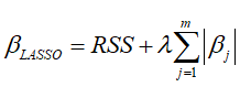
In order to overcome the cons issue in Ridge Regression, the LASSO is introduced with the similar shrinkage parameter, but the different is not in square term of the coefficient but only absolute value
Similar to Ridge Regression, LASSO also shrink the coefficient, but force coefficients to be equal to 0. Making it ability to perform feature selection
In statistics the coefficient esimated produced by this method is know as L1 norm

9.2.1 Implementation

cvfit_LASSO    <- cv.glmnet(x,y,alpha=1)
plot(cvfit_LASSO)

log(cvfit_LASSO$lambda.min)
log(cvfit_LASSO$lambda.1se)

coef(cvfit_LASSO,s=cvfit_LASSO$lambda.min)
coef(cvfit_LASSO,s=cvfit_LASSO$lambda.1se)

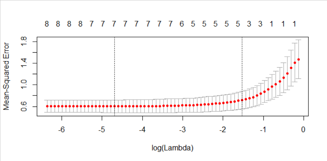
The plot shows the Mean Square Error based on training model with 𝜆 variation.
Top of the chart shows number of predictors used. Now instead of showing all 8 predictors as in Ridge Regression, LASSO shows the different number of predictors as MSE values change.
Similar to RR, there are 2 𝜆 values: (1) 𝜆.min which can be computed using log(cvfit_LASSO$lambda.min) and (2) 𝜆.1se (1 standard error from min value) which can be computed using log(cvfit_LASSO$lambda.1se)
The corresponding β values for each predictors can be found using coef(cvfit_Ridge,s=cvfit_LASSO$lambda.1se) or coef(cvfit_LASSO,s=cvfit_Ridge$lambda.min)

Fit_LASSO <- glmnet(x,y,alpha=1)
plot_glmnet(Fit_LASSO,label=TRUE,xvar="lambda",
            col=seq(1,8),,grid.col = 'lightgray')

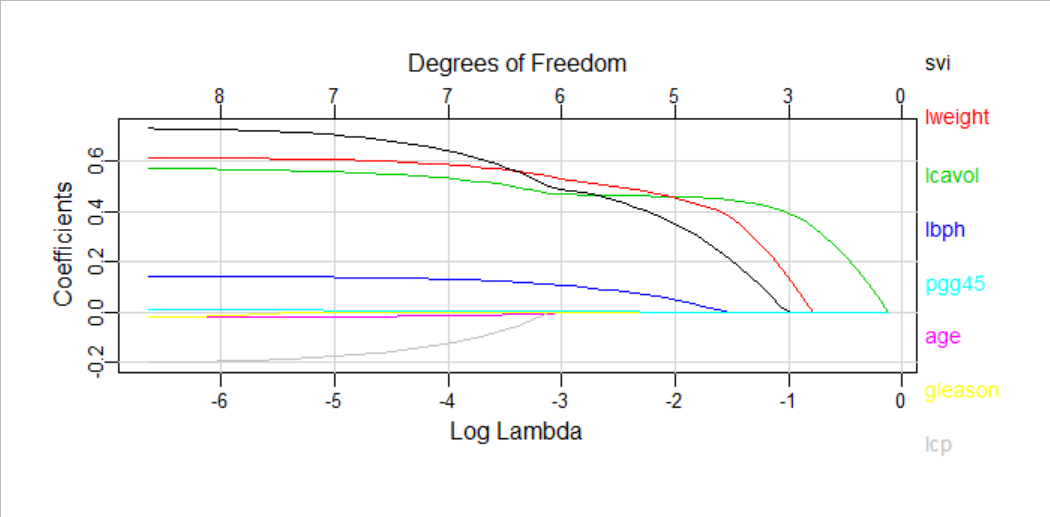The plot shows different coefficients for all predictors with 𝜆 variation. Depending on 𝜆 values that the β varying and it can be 0 at certain point.

Using 𝜆.1se, we obtain reasonable result:

> predict_LASSO <- predict(cvfit_LASSO,newx=xtest,s="lambda.1se")
> postResample(predict_LASSO,testing$lpsa)
     RMSE  Rsquared       MAE 
0.6783357 0.6096333 0.5030956 

9.3 Elastic Nets

Elastic Nets Regularization is a method that includes both LASSO and Ridge Regression. Its formulation for the loss function is as following:

𝛼=0: pure Ridge Regression
𝛼=1: pure LASSO
0<𝛼<1: Elastic Nets

9.3.1 Implementation

cvfit_ELN    <- cv.glmnet(x,y,alpha=0.5)
plot(cvfit_ELN)

Key Points

Regularization, Ridge Regression, LASSO, Elastic Nets

Dimension Reduction

Overview

Teaching: 20 min
Exercises: 0 min

Questions

What happen when there are lots of covariates?

Objectives

Learn how to apply PCA in ML model

10 Principal Component Analysis

Handy with large data
Where many variables correlate with one another, they will all contribute strongly to the same principal component
Each principal component sums up a certain percentage of the total variation in the dataset
More Principal Components, more summarization of the original data sets

10.1 Explanation

For example, we have 3 data sets: X, Y, Z
We need to compute the covariance matrix M for the 3 data set:

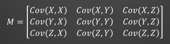
in which, the covariance value between 2 data sets can be computed as:

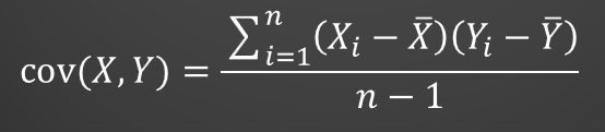
For the Covariance matrix M, we will find m eigenvectors and m eigenvalues

- Given mxm matrix, we can find m eigenvectors and m eigenvalues
- Eigenvectors can only be found for square matrix.
- Not every square matrix has eigenvectors
- A square matrix A and its transpose have the same eigenvalues but different eigenvectors
- The eigenvalues of a diagonal or triangular matrix are its diagonal elements.
- Eigenvectors of a matrix A with distinct eigenvalues are linearly independent.

Eigenvector with the largest eigenvalue forms the first principal component of the data set … and so on …*

10.2 Implementation

10.2.1 Compute PCA using eigenvector:

library(PerformanceAnalytics)
data(mtcars)
#Ignore vs & am (PCA works good with numeric data )
datain <- mtcars[,c(1:7,10:11)]
chart.Correlation(datain)
cin <- cov(scale(datain))
ein <- eigen(cin)
newpca <-   -scale(datain) %*% ein$vectors

10.2.2 Compute PCA using built-in function:

mtcars.pca <- prcomp(datain,center=TRUE,scale=TRUE)
summary(mtcars.pca)

10.2.3 A nice way to plot PCA:

Install ggbiplot package:

library(devtools)
install_github("vqv/ggbiplot")

library(ggbiplot)
ggbiplot(mtcars.pca)
ggbiplot(mtcars.pca, labels=rownames(mtcars))
ggbiplot(mtcars.pca,ellipse=TRUE,  labels=rownames(mtcars))

mtcars.country <- c(rep("Japan", 3), rep("US",4), rep("Europe", 7),rep("US",3), "Europe", rep("Japan", 3), rep("US",4), rep("Europe", 3), "US", rep("Europe", 3))

ggbiplot(mtcars.pca,ellipse=TRUE,labels=rownames(mtcars),groups = mtcars.country)

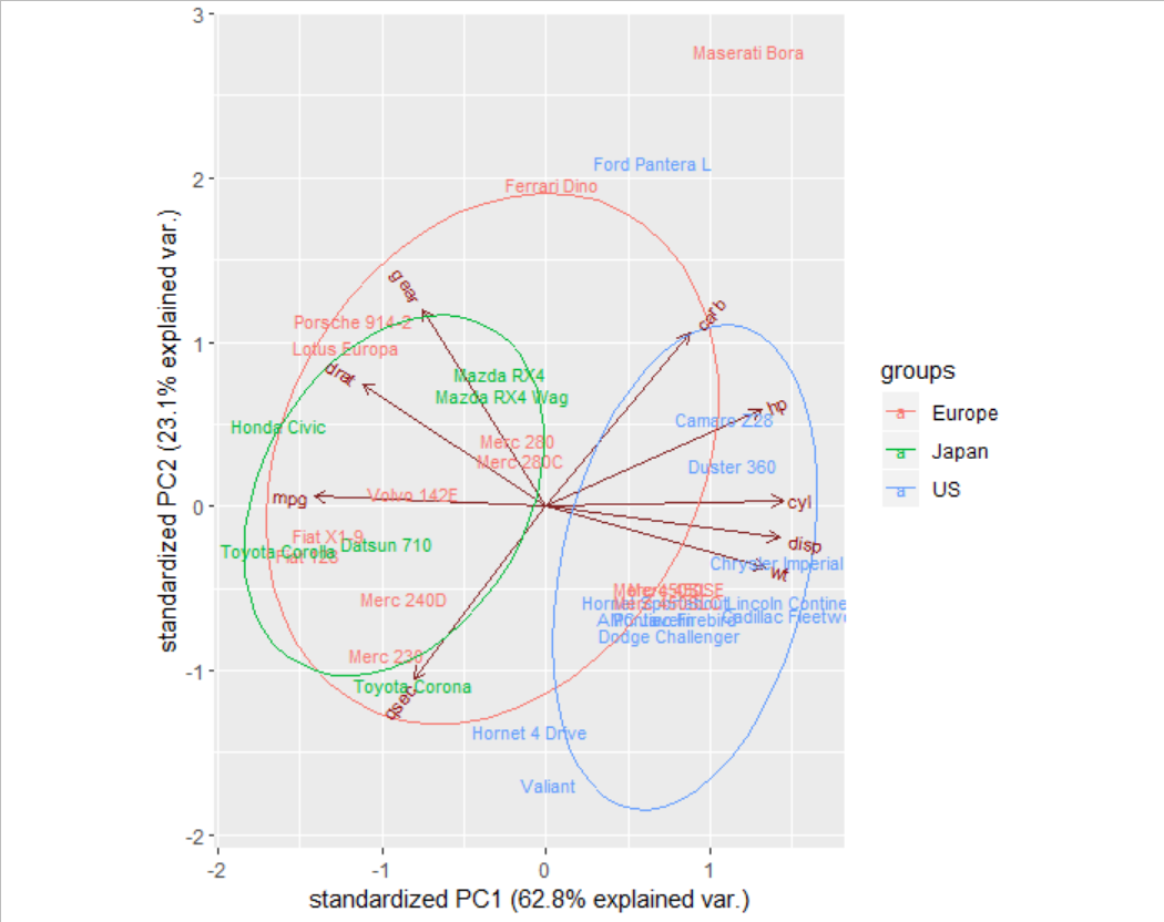
10.2.4 Application of PCA model in Machine Learning:

data(mtcars)
set.seed(123)
datain <- mtcars[,c(1:7,10:11)]

indT <- createDataPartition(y=datain$mpg,p=0.6,list=FALSE)
training <- datain[indT,]
testing  <- datain[-indT,]

preProc <- preProcess(training[,-1],method="pca",pcaComp = 1)
trainPC <- predict(preProc,training[,-1])
testPC  <- predict(preProc,testing[,-1])

traindat<- cbind(training$mpg,trainPC)
testdat <- cbind(testing$mpg,testPC)

names(traindat) <- c("mpg","PC1")
names(testdat)  <- names(traindat) 

modFitPC<- train(mpg~.,method="lm",data=traindat)

predictand <- predict(modFitPC,testdat)
postResample(testing$mpg,as.vector(predictand))

Key Points

PCA

Neural Network

Overview

Teaching: 20 min
Exercises: 0 min

Questions

How to use Neural Network in Machine Learning model

Objectives

Learn how to use ANN in ML model

11 Neural Network

Formulation of Neural Network

Here, x1,x2....xn are input variables. w1,w2....wn are weights of respective inputs.
b is the bias, which is summed with the weighted inputs to form the net inputs. 
Bias and weights are both adjustable parameters of the neuron.
Parameters are adjusted using some learning rules. 
The output of a neuron can range from -inf to +inf.
The neuron doesn’t know the boundary. So we need a mapping mechanism between the input and output of the neuron. 
This mechanism of mapping inputs to output is known as Activation Function.

Activation functions:
Neural Network formulation

Basic Type of Neural Network:

11.1 Implementation

install.packages("neuralnet")

Split the data

library(caret)
library(neuralnet)

datain <- mtcars
set.seed(123)
#Split training/testing
indT <- createDataPartition(y=datain$mpg,p=0.6,list=FALSE)
training <- datain[indT,]
testing  <- datain[-indT,]
#scale the data set
smax <- apply(training,2,max)
smin <- apply(training,2,min)
trainNN <- as.data.frame(scale(training,center=smin,scale=smax-smin))
testNN <- as.data.frame(scale(testing,center=smin,scale=smax-smin))

Fit the Neural Network using 1 hidden layer with 10 neurons using backpropagation:

set.seed(123)
ModNN <- neuralnet(mpg~cyl+disp+hp+drat+wt+qsec+carb,trainNN, hidden=10,linear.output = T)
plot(ModNN)

#Predict using Neural Network
predictNN <- compute(ModNN,testNN[,c(2:7,11)])
predictmpg<- predictNN$net.result*(smax-smin)[1]+smin[1]
postResample(testing$mpg,predictmpg)
   RMSE  Rsquared       MAE 
3.0444857 0.8543388 2.3276645 

Key Points

ANN

Support Vector Machine

Overview

Teaching: 20 min
Exercises: 0 min

Questions

How to use Support Vector Machine in Machine Learning model

Objectives

Learn how to use SVM in ML model

12 Support Vector Machine

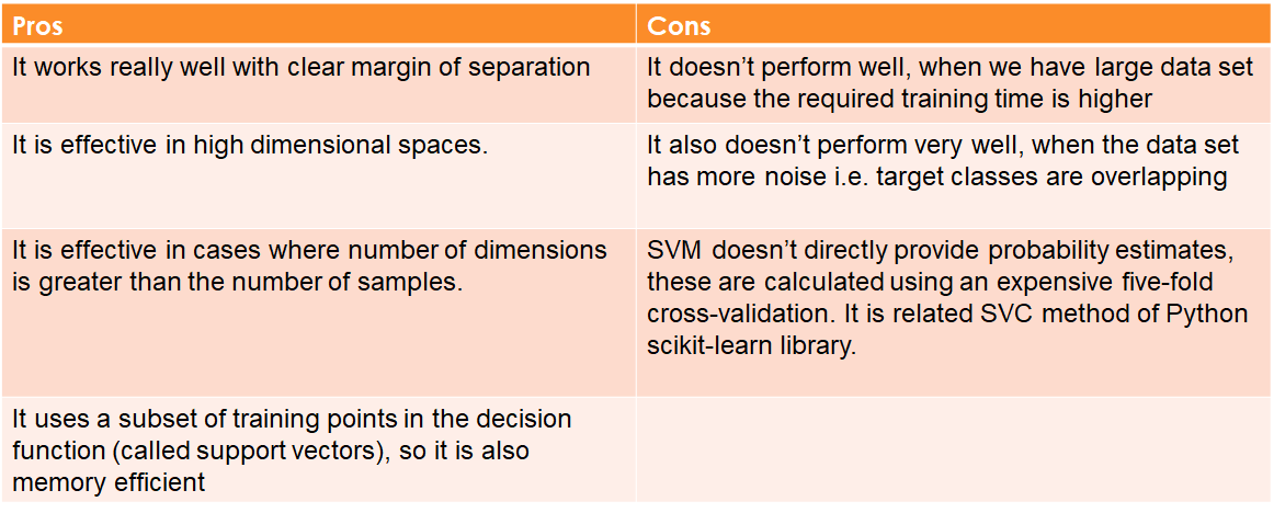
The objective of the support vector machine (SVM) algorithm is to find a hyperplane in an N-dimensional space that distinctly classifies the data points.

12.1 Applications of Support Vector Machine:

12.2 Explanation

To separate the two classes of data points, there are many possible hyperplanes that could be chosen

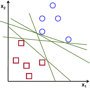
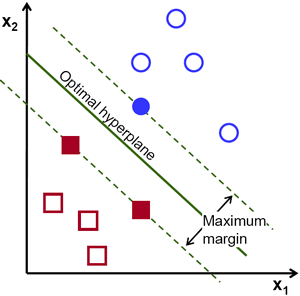
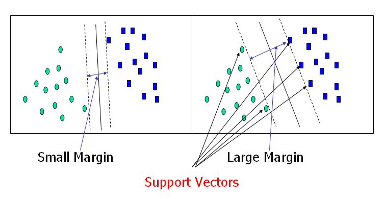
SVM’s objective is to find a plane that has the maximum margin, i.e the maximum distance between data points of both classes. Maximizing the margin distance provides some reinforcement so that future data points can be classified with more confidence.

Example of hyperplane in 2D and 3D position:

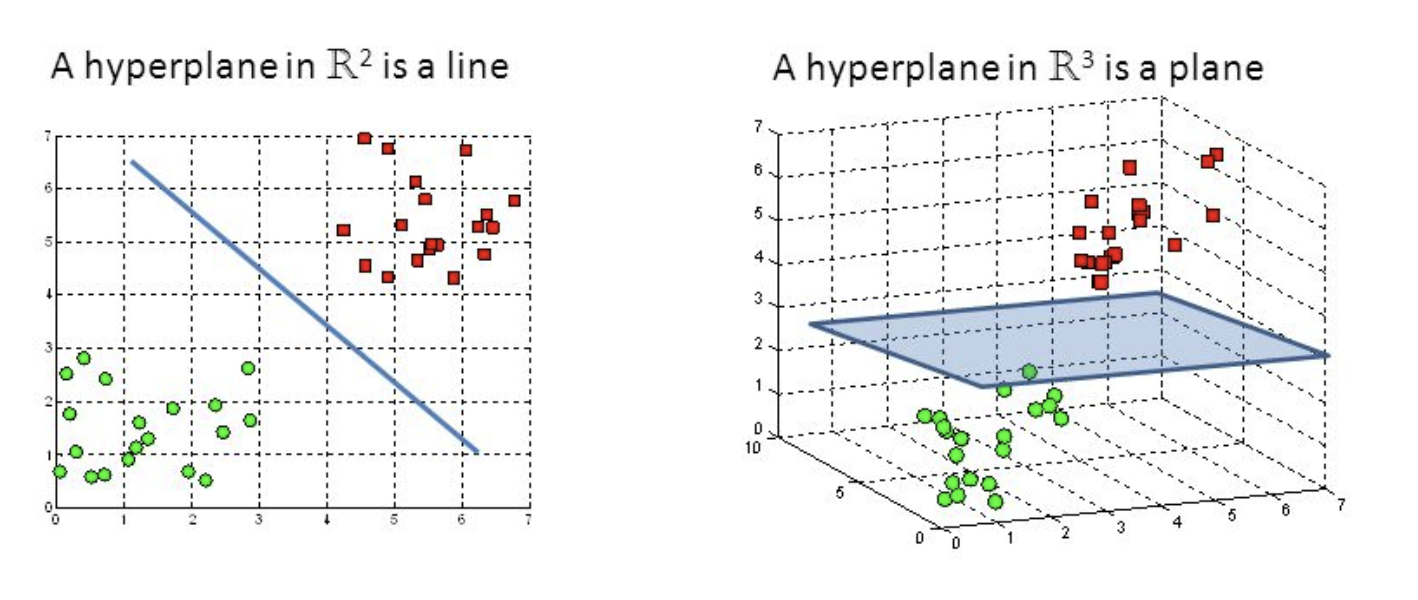
Support vectors (SVs) are data points that are closer to the hyperplane and influence the position and orientation of the hyperplane. Using SVs to maximize the margin of the classifier. Removing SVs will change the position of the hyperplane. These are the points that help us build our SVM.

12.3 Implementation

Using caret package:

library(caret)
indT <- createDataPartition(y=iris$Species,p=0.6,list=FALSE)
training <- iris[indT,]
testing  <- iris[-indT,]

ModFit_SVM <- train(Species~.,training,method="svmLinear",preProc=c("center","scale"))
predict_SVM<- predict(ModFit_SVM,newdata=testing)
confusionMatrix(testing$Species,predict_SVM)

Note: there are other function in method = “svmPoly”, “svmRadial”, “svmRadialCost”, “svmRadialSigma”

Using e1071 package, we have better demonstration:

library(e1071)
Fit_SVM_ln <- svm(Species~Petal.Width+Petal.Length,
               data=training,kernel="sigmoid")
plot(Fit_SVM_ln,training[,3:5])

Fit_SVM_rbg <- svm(Species~Petal.Width+Petal.Length,
               data=training,kernel="radial",gamma=0.1)
plot(Fit_SVM_rbg,training[,3:5])

pred_rbg <- predict(Fit_SVM_ln,testing)
confusionMatrix(testing$Species,pred_rbg)

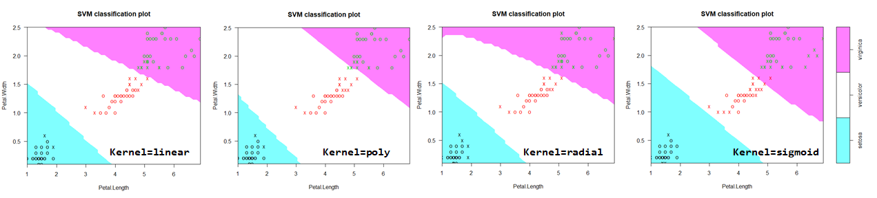
Using different gamma parameter for kernal radial:

Fit_SVM_rbg <- svm(Species~Petal.Width+Petal.Length,
             data=training,kernel="radial",gamma=0.1)
plot(Fit_SVM_rbg,training[,3:5])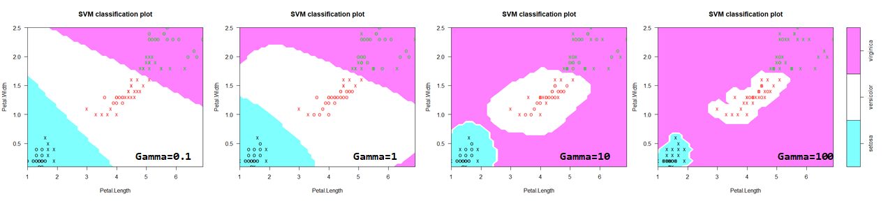

Key Points

SVM

K-Nearest Neighbour

Overview

Teaching: 20 min
Exercises: 0 min

Questions

How to use K-Nearest Neighbour in Machine Learning model

Objectives

Learn how to use KNN in ML model

13 K-Nearest Neighbour

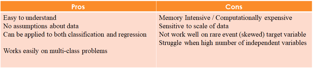
Simplicity but powerful and fast for certain task
Work for both classification and regression
Named as Instance Based Learning; Non-parametrics; Lazy learner
Work well with small number of inputs

13.1 Explanation

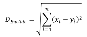
In KNN, the most important parameter is the K group and the distance computed between points.
Euclide distance:

13.2 Implementation

library(caret)
data(iris)
set.seed(123)
indT <- createDataPartition(y=iris$Species,p=0.6,list=FALSE)
training <- iris[indT,]
testing  <- iris[-indT,]

ModFit_KNN <- train(Species~.,training,method="knn",preProc=c("center","scale"),tuneLength=20)

ggplot(ModFit_KNN$results,aes(k,AccuracySD))+
      geom_point(color="blue")+
      labs(title=paste("Optimum K is ",ModFit_KNN$bestTune),
           y="Error")
      
predict_KNN<- predict(ModFit_KNN,newdata=testing)
confusionMatrix(testing$Species,predict_KNN)

Key Points

KNN

Unsupervised Learning

Overview

Teaching: 20 min
Exercises: 0 min

Questions

What is Unsupervised Learning in Machine Learning model

Objectives

Learn how to use K-mean clustering in ML model

14 Unsupervised Learning

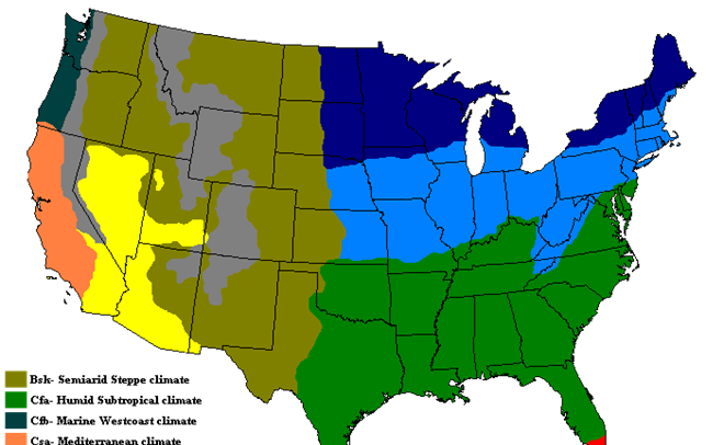
Used when no feature output data
Often used for clustering data

Typical method:

K-means clustering
Hierarchical clustering
Ward clustering
Partition Around Median (PAM)

14.1 K-means clustering

14.1.1 Explanation of K-means clustering method:

Given a set of data, we choose K=2 clusters to be splited:

First select 2 random centroids (denoted as red and blue X)

Compute the distance between 2 centroid red X and blue X with all the points (for instance using Euclidean distance) and compare with each other. 2 groups are created with shorter distance to 2 centroids

Now recompute the new centroids of the 2 groups (using mean value of all points in the same groups):

Compute the distance between 2 new centroids and all the points. We have 2 new groups:

Repeat the last 2 steps until no more new centroids created. The model reach equilibrium:

14.1.2 Example with K=3

14.1.3 Implementation

library(ggplot2)
library(factoextra)
library(purrr)
data(iris)
ggplot(iris,aes(x=Sepal.Length,y=Petal.Width))+
      geom_point(aes(color=Species))
set.seed(123)
km <- kmeans(iris[,3:4],3,nstart=20)

table(km$cluster,iris$Species)
fviz_cluster(km,data=iris[,3:4])

14.1.4 How to find optimal K values:

14.1.4.1 Elbow approach

Similar to KNN method for supervised learning, for K-means approach, we are able to use Elbow approach to find the optimal K values.
The Elbow approach ues the Within-Cluster Sum of Square (WSS) to measure the compactness of the clusters:

The optimal K-values can be found from the Elbow using method=”wss”:

fviz_nbclust(iris[,3:4], kmeans, method = "wss")

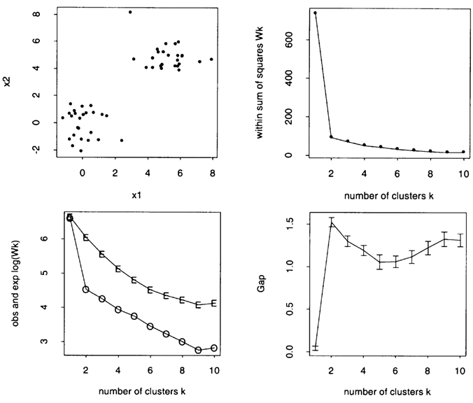
14.1.4.2 Gap-Statistics approach

Developed by Prof. Tibshirani et al in Stanford
Applied to any clustering method (K-means, Hierarchical)
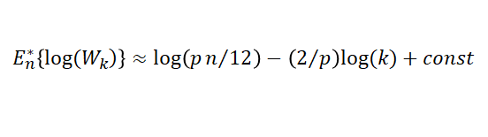
Maximize the Gap function:

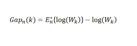
E*n: expectation under a sample size of n from the reference distribution

library(cluster)
# B is number of Monte Carlo bootstrap samples
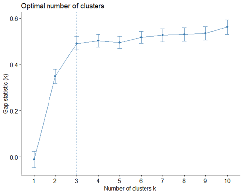
gap_stat <- clusGap(iris[,3:4], FUN = kmeans, nstart=20, K.max = 10, B = 50)
fviz_gap_stat(gap_stat)

Key Points

K-mean

Mini-Project

Overview

Teaching: 10 min
Exercises: 180 min

Questions

What do you learn from Machine Learning workshop using R caret?

Objectives

Learn how to apply Machine Learning into your real project

15. MINI PROJECT

Description of Mini Project:

This Mini Project evaluates the ability of you working on a sample Data Science project from scratch.
The project is about Supervised Machine Learning only
It requires you to download data, clean data, split into training/testing and apply any machine learning model and analyse the output.

Requirement:

You can write the script in RStudio (on Palmetto’s Open OnDemand or your PCs/Macs) and save it as your_username.R and send it to my email: tuev@clemson.edu. You can also upload to your github page and share to me
Note: in order to get the Certificate of Attendence, you should send me the R script on or before 09/30/2021.

Data

You can use any data in your field of expertise (most preferred method). If so, please send along the dataset with the Rscript
You can also use Kaggle data which can be found here (second preferred method). Please elaborate in the ipynb how did you retrieve the data
You can use use Titanic data from our repo. Description for Titanic data can be found here (third preferred method)

Method

In the R solution file I would like to see the following:

Clearly state the objective of the mini-project on Supervised Machine Learning
Brief explanation about the data that you will be using: source, predictors, predictand
Type of ML model output: Continuous or Classification?
Read in the data
Clean & Standardized the input data if needed
Split data to training/testing (You can also use Cross Validation if needed, not required)
You can use any Regularization (variable selection) or PCA if needed (not required)
Construct Machine Learning model to training set and explain why do you want to use that algorithm (any model is fine for me)
Apply Machine Learning model to predict the output from testing set
Evaluate the output using any of the given method in chapter 4
Confirm if your ML model is good or bad?

Key Points

Self-project

Introduction to Machine Learning using R

Introduction to Machine Learning

Overview

Key Points

Introduction to Caret

Overview

2.1 What is Caret

2.2 Why using Caret

2.3 Install caret

2.4 Pre-processing using caret

2.4.1 Visualize important variables

2.4.2 Pre-processing with missing value

Key Points

Data Partition with caret

Overview

3 Data partition: training and testing

3.1 Data spliting using Data Partition

3.2 Data spliting using K-fold: Cross validation approach

3.3 Other Cross-Validation approach

Key Points

Evaluation Metrics with caret

Overview

4 Evaluation Metrics

4.1 Regression model Evaluation Metrics

4.1.1 Correlation Coefficient (R) or Coefficient of Determination (R2):

4.1.2 Root Mean Square Error (RMSE) or Mean Square Error (MSE)

4.2. Classification model Evaluation Metrics

4.2.1 Confusion Matrix

Key Points

Training Machine Learning model using Regression Method

Overview

5 Supervised Learning training

5.1 For Continuous output

5.1.1 Train model using Linear Regression

5.1.2 Train model using Multi-Linear Regression

5.1.3 Train model using Stepwise Linear Regression

5.1.4 Train model using Polynomial Regression

5.1.5 Train model using Principal Component Regression

5.2 For categorical output

5.2.1 Train model using Logistic Regression

Key Points

Training Machine Learning model using Tree-based model

Overview

Supervised Learning training

Train model using Decision Tree

Spliting algorithm

Pros & Cons

Implementation

Train model using Random Forest

Detail explaination

Pros & Cons of Random Forest

Implementation of Random Forest

Key Points

Training Machine Learning model using Ensemble approach

Overview

7.1 Why Ensemble:

7.2 Train model using Ensemble Approach

7.3 Train model using Bagging (Bootstrap Aggregation)

7.3.1 Detail explaination of Bagging

7.3.2 Implementation of Bagging using decision Tree

7.4 Train model using Boosting

7.4.1 Adaptive Boosting: Adaboost

7.4.2 Gradient Boosting Machines:

7.5 Compare Bagging and Boosting technique:

7.6 Conclusions

Key Points

Training Machine Learning model using Model based Prediction

Overview

8.1 Naive Bayes

8.1 Implementation Naive Bayes

8.2 Linear Discriminent Analysis

8.2.1 Implementation LDA

Key Points

Regularization and Variable Selection

Overview

9 Regularization

9.1 Ridge Regression

9.1.2 Implementation

9.2 LASSO: Least Absolute Shrinkage & Selection Operator

9.2.1 Implementation

2.3 Install `caret`

2.4 Pre-processing using `caret`

3.1 Data spliting using `Data Partition`

3.2 Data spliting using `K-fold`: Cross validation approach