Introduction to Spatial Vector data

Overview

Teaching: 20 min
Exercises: 0 min

Questions

• What is Geospatial Vector data

Objectives

• Describe the characteristics of 3 key vector data structures: points, lines and polygons.

• Open a shapefile in Python using geopandas - gpd.read_file().

• View the CRS and other spatial metadata of a vector spatial layer in Python

• Access and view the attributes of a vector spatial layer in Python.

2.1 Geospatial Vector data

Vector data

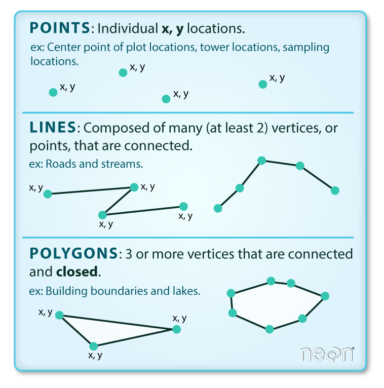
Vector data are composed of discrete geometric locations (x, y values) known as vertices that define the “shape” of the spatial object. The organization of the vertices determines the type of vector that you are working with. There are three types of vector data:

• Points: Each individual point is defined by a single x, y coordinate. There can be many points in a vector point file. Examples of point data include: sampling locations, the location of individual trees or the location of plots.

• Lines: Lines are composed of many (at least 2) vertices, or points, that are connected. For instance, a road or a stream may be represented by a line. This line is composed of a series of segments, each “bend” in the road or stream represents a vertex that has defined x, y location.

• Polygons: A polygon consists of 3 or more vertices that are connected and “closed”. Thus the outlines of plot boundaries, lakes, oceans, and states or countries are often represented by polygons. Occasionally, a polygon can have a hole in the middle of it (like a doughnut), this is something to be aware of but not an issue you will deal with in this tutorial.

Shapefiles

• Geospatial data in vector format are often stored in a shapefile_ format. Because the structure of points, lines, and polygons are different, each individual shapefile can only contain one vector type (all points, all lines or all polygons). You will not find a mixture of point, line and polygon objects in a single shapefile.

• Objects stored in a shapefile often have a set of associated attributes that describe the data. For example, a line shapefile that contains the locations of streams, might contain the associated stream name, stream “order” and other information about each stream line object.

Shapefile structures

• A shapefile is created by 3 or more files, all of which must retain the same NAME and be stored in the same file directory, in order for you to be able to work with them.
• There are 3 key files associated with any and all shapefiles:

  .shp: the file that contains the geometry for all features.
  .shx: the file that indexes the geometry.
  .dbf: the file that stores feature attributes in a tabular format.
  

Sometimes, a shapefile will have other associated files including:

.prj: the file that contains information on projection format including the coordinate system and projection information. It is a plain text file describing the projection using well-known text (WKT) format.
.sbn and .sbx: the files that are a spatial index of the features.
.shp.xml: the file that is the geospatial metadata in XML format, (e.g. ISO 19115 or XML format).

Data Management - Sharing Shapefiles

When you work with a shapefile, you must keep all of the key associated file types together. And when you share a shapefile with a colleague, it is important to zip up all of these files into one package before you send it to them!

2.2 Working with Shapefile using Python

Download Shapefiles

You will use the geopandas library to work with vector data in Python. You will also use matplotlib.pyplot to plot your data.

First import library and download data:

# Import packages
import os
import matplotlib.pyplot as plt
import geopandas as gpd
import earthpy as et

# Get data and set working directory
data = et.data.get_data('spatial-vector-lidar')
os.chdir(os.path.join(et.io.HOME, 'earth-analytics'))

The data is downloaded to your home directory:

$HOME/earth-analytics/data/spatial-vector-lidar/

Open and Read shapefiles

The shapefiles that you will import are:

• A polygon shapefile representing our field site boundary,
• A line shapefile representing roads, and
• A point shapefile representing the location of field sites at the San Joachin field site.

The first shapefile that you will open contains the point locations of plots where trees have been measured. To import shapefiles you use the geopandas function read_file(). Notice that you call the read_file() function using _gpd.read_file() _to tell python to look for the function within the geopandas library.

# Define path to file
path1 = "data/spatial-vector-lidar/california/neon-sjer-site/vector_data/"

# Import shapefile using geopandas
sjer_locations = gpd.read_file(path1+"SJER_plot_centroids.shp")

Spatial Data Attributes

Each object in a shapefile has one or more attributes associated with it. Shapefile attributes are similar to fields or columns in a spreadsheet. Each row in the spreadsheet has a set of columns associated with it that describe the row element. In the case of a shapefile, each row represents a spatial object - for example, a road, represented as a line in a line shapefile, will have one “row” of attributes associated with it. These attributes can include different types of information that describe objects stored within a shapefile. Thus, our road, may have a name, length, number of lanes, speed limit, type of road and other attributes stored with it.

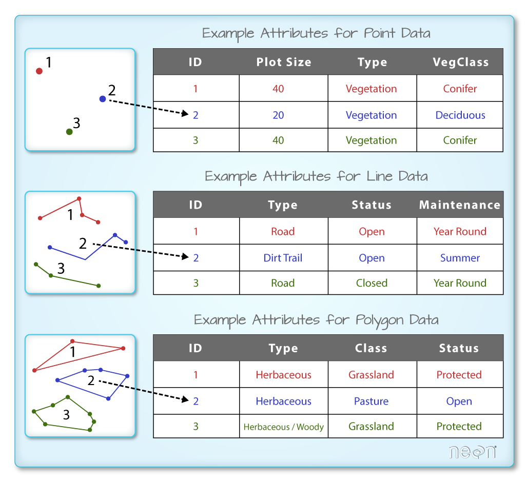
You can use the .head(3) function to only display the first 3 rows of the attribute table. The number in the .head() function represents the total number of rows that will be returned by the function.

sjer_locations.head(3)

In this case, you have several attributes associated with our points including:

sjer_locations.columns

Spatial Metadata

Key metadata for all shapefiles include:

• Object Type: the class of the imported object.

sjer_locations.geom_type

• Coordinate Reference System (CRS): the projection of the data.

sjer_locations.crs

• Extent: the spatial extent (geographic area that the shapefile covers) of the shapefile. Note that the spatial extent for a shapefile represents the extent for ALL spatial objects in the shapefile.

sjer_locations.total_bounds

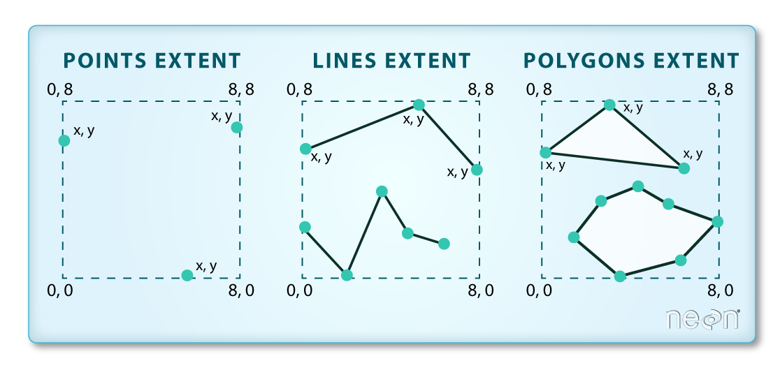(The spatial extent of a shapefile or geopandas GeoDataFrame represents the geographic “edge” or location that is the furthest north, south east and west. Thus is represents the overall geographic coverage of the spatial object)

How many features in your Shapefiles?

You can view the number of features (counted by the number of rows in the attribute table) and feature attributes (number of columns) in our data using the pandas .shape method. Note that the data are returned as a vector of two values:

sjer_locations.shape

2.3. Plot a point Shapefile

Quick plotting

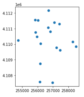
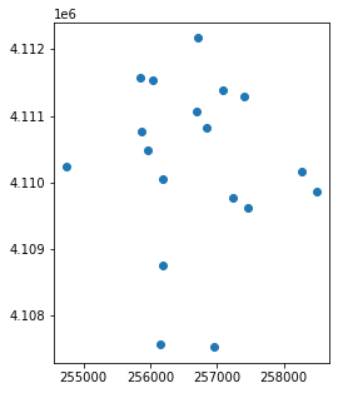
Next, you can visualize the data in your Python geodataframe object using the .plot() method. Notice that you can create a plot using the geopandas base plotting using the syntax:

sjer_locations.plot()

Plotting in axis object

However in general it is good practice to setup an axis object so you can plot different layers together (similar to subplot). When you do that you need to provide the plot function with the axis object that you want it to plot on.

You then plot the data and provide the ax= argument with the ax object.

fig, ax = plt.subplots(figsize=(5, 5))

# Plot the data using geopandas .plot() method
sjer_locations.plot(ax=ax)

plt.show()

Changing colormap, marker,

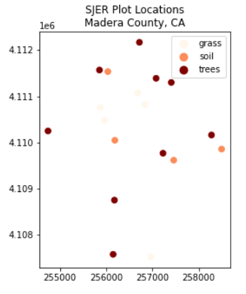
You can plot the data by feature attribute and add a legend too. Below you add the following plot arguments to your geopandas plot:

• column: the attribute column that you want to plot your data using
• categorical=True: set the plot to plot categorical data - in this case plot types.
• legend: add a legend
• markersize: increase or decrease the size of the points or markers rendered on the plot
• cmap: set the colors used to plot the data
• title add a title to your plot.

and fig size if you want to specify the size of the output plot.

fig, ax = plt.subplots(figsize=(5, 5))

sjer_plot_locations.plot(column='plot_type',
                         categorical=True,                         
                         marker='*',
                         markersize=45,
                         cmap='OrRd', 
                         legend=True,
                         ax=ax)
                         

ax.set_title('SJER Plot Locations\nMadera County, CA')

plt.show()

2.4

2.5 Ploting Polygon shapefiles

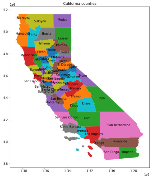
Here we plot different counties in California

# Define path to file
path2 = "data/spatial-vector-lidar/california/CA_Counties/"

# Import shapefile using geopandas
CA_Counties = gpd.read_file(path2+"CA_Counties_TIGER2016.shp")
CA_Counties.head()

Let’s plot county by name with text label

# Create coords column from geometry column
CA_Counties['coords'] = CA_Counties['geometry'].apply(lambda x: x.representative_point().coords[:])
CA_Counties['coords'] = [coords[0] for coords in CA_Counties['coords']]

# Plot 2D plot
fig,ax = plt.subplots(figsize=(10,10))
CA_Counties.plot(column="NAME",ax=ax)
ax.set(title="California counties")

for idx, row in CA_Counties.iterrows():
    plt.annotate(text=row['NAME'], xy=row['coords'],
                 horizontalalignment='center')

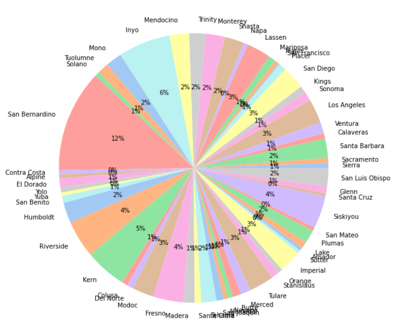
We create a new column name ATotal(%) which the total counties area in percentage vs the whole CA State

Total_Land = CA_Counties['ALAND'].sum()+CA_Counties['AWATER'].sum()
CA_Counties['ATotal(%)']=(CA_Counties['ALAND']+CA_Counties['AWATER'])/Total_Land*100

Then plot it in Pie Chart:

Plot CA Counties

fig,ax = plt.subplots(figsize=(10,10))

#create pie chart
colors = sns.color_palette('pastel')[0:100]

plt.pie(CA_Counties["ATotal(%)"], labels = CA_Counties["NAME"], colors = colors, autopct='%.0f%%')
plt.show()

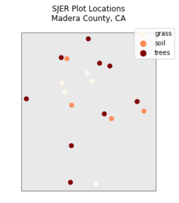
2.6 Plot Multiple Shapefiles Together With Geopandas

You can plot several layers on top of each other using the geopandas .plot method. To do this, you:

• Define the ax variable just as you did above to add a title to our plot.
• Add as many layers to the plot as you want using geopandas .plot() method.

Notice below

• ax.set_axis_off() is used to turn off the x and y axis and
• plt.axis(‘equal’) is used to ensure the x and y axis are uniformly spaced.

# Import crop boundary using geopandas
sjer_crop_extent = gpd.read_file(path1+"SJER_crop.shp")

# Now plot these 2 shapefiles using the same axis
fig, ax = plt.subplots(figsize=(5, 5))

# First setup the plot using the crop_extent layer as the base layer
sjer_crop_extent.plot(color='lightgrey',
                      edgecolor='black',
                      alpha=.5,
                      ax=ax)

# Add another layer using the same ax
sjer_locations.plot(column='plot_type',
                         categorical=True,
                         marker='o',
                         markersize=45,
                         cmap='OrRd', 
                         legend=True,
                         ax=ax)

# Clean up axes
ax.set_title('SJER Plot Locations\nMadera County, CA')
ax.set_axis_off()

plt.axis('equal')
plt.show()

Key Points

• earthpy, shapefile, XML, GeoJSON