Overview

Teaching: 20 min
Exercises: 0 min

Questions

• How to train a Machine Learning model with continuos output

Objectives

• Learn to use different ML algorithm for Supervised Learning

5 Network common data NetCDF format

5.1 What is NetCDF?

NetCDF (network Common Data Form) is a hierarchical data format . It is what is known as a “self-describing” data structure which means that metadata, or descriptions of the data, are included in the file itself and can be parsed programmatically, meaning that they can be accessed using code to build automated and reproducible workflows.

The NetCDF format can store data with multiple dimensions. It can also store different types of data through arrays that can contain geospatial imagery, rasters, terrain data, climate data, and text. These arrays support metadata, making the netCDF format highly flexible. NetCDF was developed and is supported by UCAR who maintains standards and software that support the use of the format.

It is perfect to store Climate data with x and y values representing latitude and longitude location for a point or a grid cell location on the earth’s surface and time.

5.2 Tools to work with NetCDF data

Python also has several open source tools that are useful for processing netcdf files including:

• Xarray: one of the most common tools used to process netcdf data. Xarray knows how to open netcdf 4 files automatically giving you access to the data and metadata in spatial formats.
• rioxarray: a wrapper that adds spatial functionality such as reproject and export to geotiff to xarray objects.
• Regionmask: regionmask builds on top of xarray to support spatial subsetting and AOIs for xarray objects.

5.3 NetCDF in Python

Loading library

import os

import numpy as np
import pandas as pd
import matplotlib.pyplot as plt

# netCDF4 needs to be installed in your environment for this to work
import xarray as xr
import rioxarray as rxr
import seaborn as sns
import geopandas as gpd
import earthpy as et

# Optional - set your working directory if you wish to use the data
# accessed lower down in this notebook (the USA state boundary data)
os.chdir(os.path.join(et.io.HOME,
                      'earth-analytics',
                      'data'))

In this lesson you will work with historic temperature data that represents air temperature for the Continental United States (CONUS).

Open up the data online

# The (online) url for a MACAv2 dataset for max monthly temperature
data_path = "tmax.nc"

tmx  = xr.open_dataset(data_path)  
# View xarray object
tmx

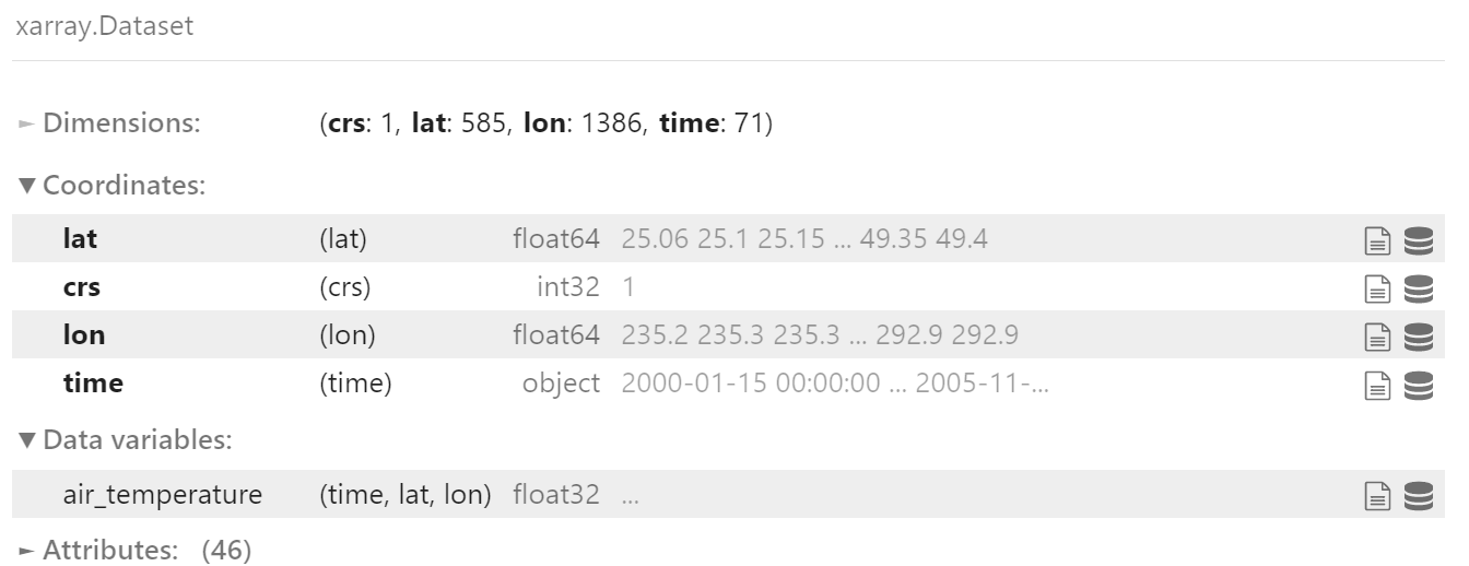
Dimensions, Variables, Attributes

From the above output, we see there are 4 Dimensions (crs: 1,lat: 585,lon: 1386,time: 71) in NetCDF file and 1 Data variable (air_temperature).

We can get the variable using the following commands:

tmx.air_temperature
# or
tmx["air_temperature"]

Next, Let’s convert temperature unit from Kelvin to Celcius

# Convert from K to C
Tc = tmx.air_temperature-273.15

# Copy attributes to get nice figure lables
Tc.attrs = tmx.air_temperature.attrs
Tc.attrs["units"]="degC"

Getting temperature from your location

Getting your location

!pip install geocoder
import geocoder
myloc = geocoder.ip('me')
my_lat,my_lon=myloc.latlng

# Convert longitude to the same longitude as NetCDF file:
my_lon =my_lon+360

print(my_lat,my_lon)

Getting the closest index to your lat/lon

indx_lat=abs((Tc.lat-my_lat)).argmin()
indx_lon=abs((Tc.lon-my_lon)).argmin()

Extract temperature data near to your location

my_tmp = Tc.isel(lat=indx_lat,lon=indx_lon)
my_tmp.plot()

Note:

• isel: index select
• sel: select any nearest value or range of value via slicing

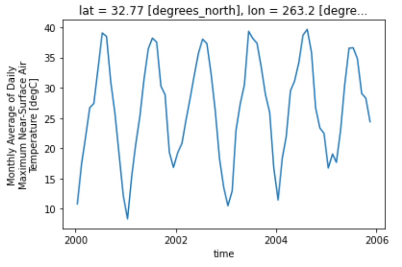
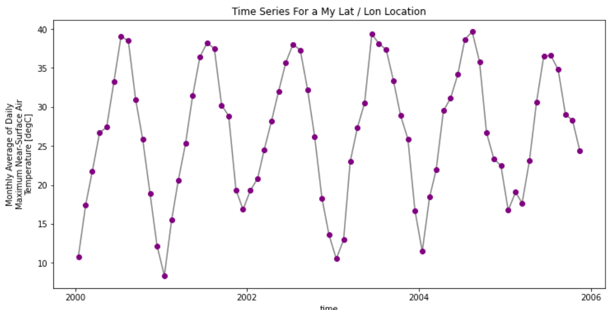
You can make the plot a bit prettier if you’d like using the standard Python matplotlib plot parameters. Below you change the marker color to purple and the lines to grey. figsize is used to adjust the size of the plot.

# You can clean up your plot as you wish using standard matplotlib approaches
f, ax = plt.subplots(figsize=(12, 6))
my_tmp.plot.line(hue='lat',
                    marker="o",
                    ax=ax,
                    color="grey",
                    markerfacecolor="purple",
                    markeredgecolor="purple")
ax.set(title="Time Series For a My Lat / Lon Location")

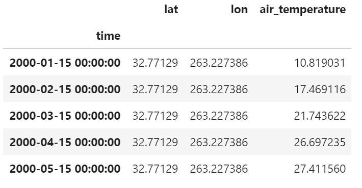
For more convinient using pandas, you can export xarray dataframe to pandas format and/or to csv:

# Convert to dataframe -- then this can easily be exported to a csv
my_tmp_df = my_tmp.to_dataframe()
# View just the first 5 rows of the data
my_tmp_df.head()

Plotting 2D map

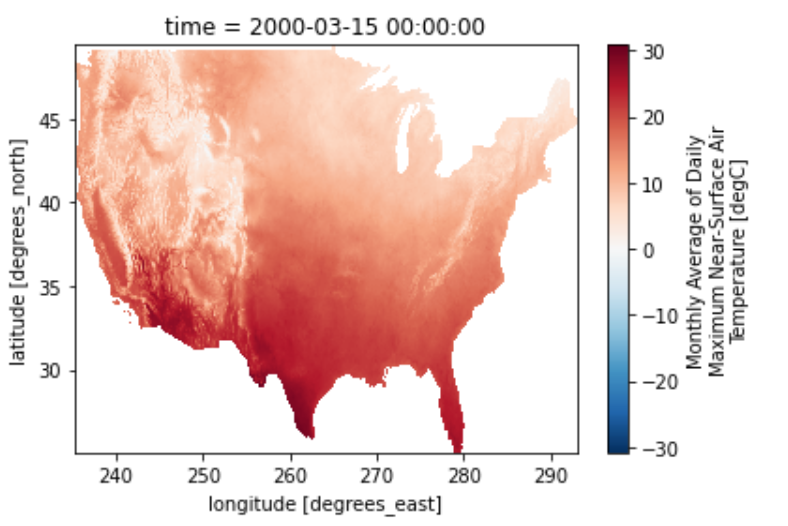
We can plot the 2D map of NetCDF with fixed time index

air2d = Tc.isel(time=2)
air2d.plot()

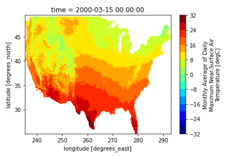
We can change the colormap as well as the number of temperature level

air2d.plot(levels=20,cmap="jet")

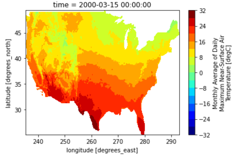
We can also smooth the pixelated map using contourf

air2d.plot.contourf(levels=20,cmap="jet")

5.4 Cropping NetCDF with shapefile

Load shapefile

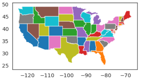
First, let open up the USA shapefile:

# Load usa shapefile
path = "/users/tuev/earth-analytics/data/spatial-vector-lidar/usa/"
usa_shp = gpd.read_file(path+"usa-states-census-2014.shp")
usa_shp.plot(column="NAME")

Select Texas state from 48 CONUS states:

TX_shp = usa_shp[usa_shp["NAME"]=="Texas"]
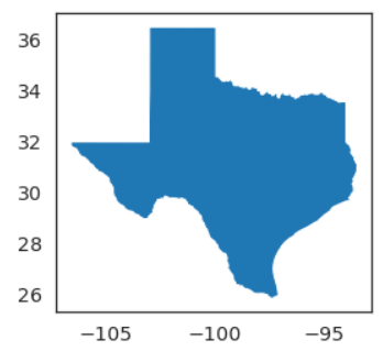
TX_shp.plot(column="NAME")

Create Texas mask from its shapefile and having the same resolution as max_temp_xr

import regionmask
TX_mask = regionmask.mask_3D_geopandas(TX_shp,
                                       air2d.lon,
                                       air2d.lat).squeeze()
                                       
TX_air_temp = Tc.where(TX_mask)

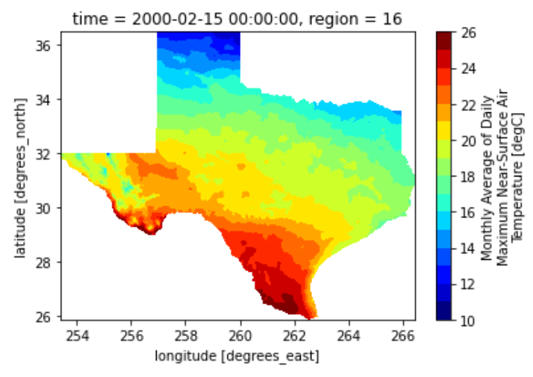
Plotting TX temperature at selected time scale

lon_min,lat_min,lon_max,lat_max = TX_shp.total_bounds
Tsel = TX_air_temp.sel(time='2000-02-15 00:00:00',
                lon =slice(lon_min+360,lon_max+360),
                lat =slice(lat_min,lat_max)).squeeze()
Tsel.plot.contourf(levels=20,cmap='jet')

Key Points

• Supervised Learning with continuous output