Overview

Teaching: 20 min
Exercises: 0 min

Questions

• How to train a Machine Learning model using Regression method

Objectives

• Learn to use different Regression algorithm for Machine Learning training

5 Supervised Learning training with Continuous output

Here we use the R sampled data named airquality with some missing values.

data(airquality)

5.1 Pre-processing data and treat missing value

Check missing value

sum(is.na(airquality))

Impute missing value using Bagging approach

PreImputeBag <- preProcess(airquality,method="bagImpute")
airquality_imp <- predict(PreImputeBag,airquality)

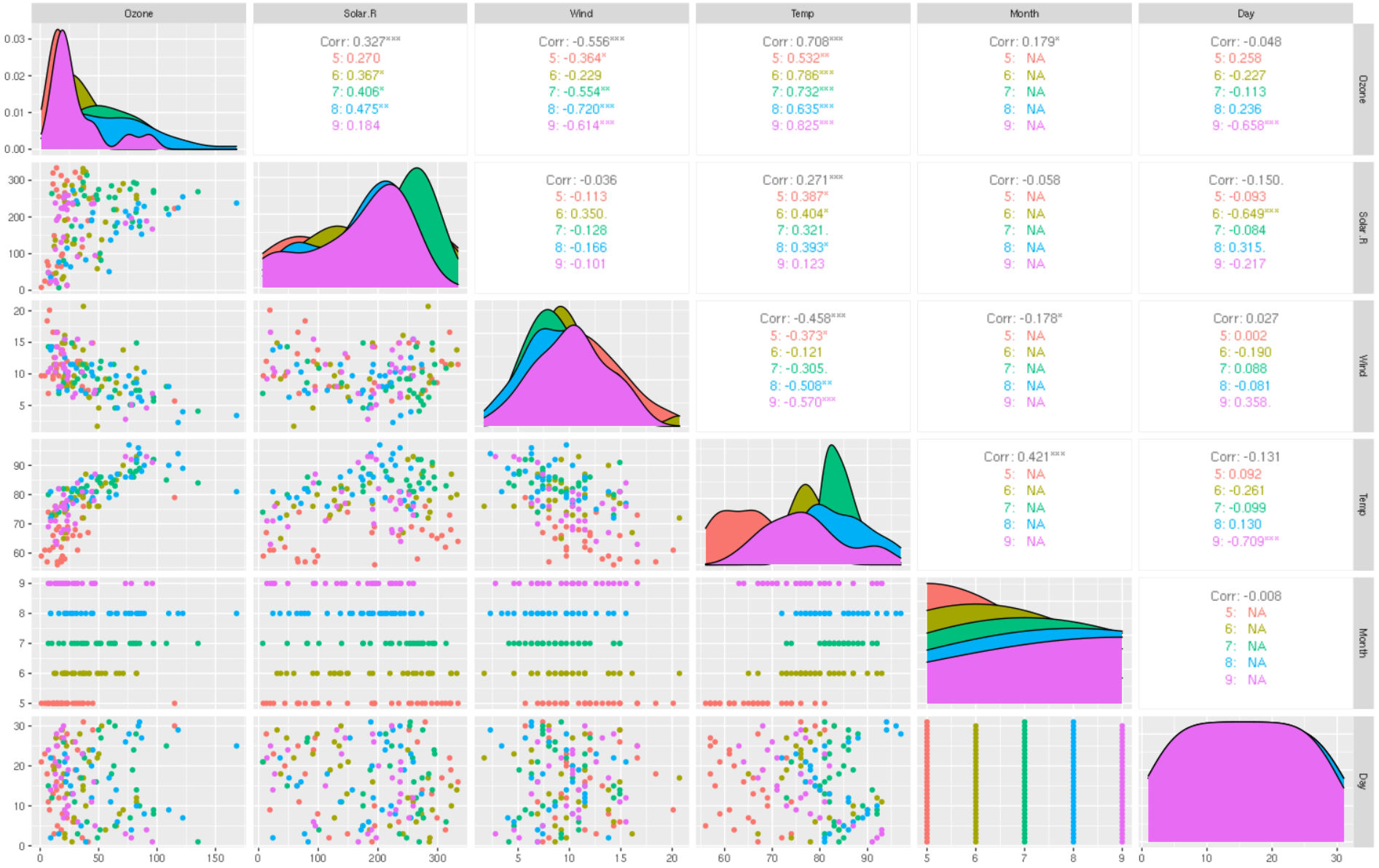
5.2 Visualize the important data

library(GGally)
ggpairs(airquality_imp,aes(colour=factor(Month)))

5.3 Split data into training and testing

indT <- createDataPartition(y=airquality_imp$Ozone,p=0.6,list=FALSE)
training <- airquality_imp[indT,]
testing  <- airquality_imp[-indT,]

Let’s use all inputs data (except Month/Day) for modeling

5.4 Train model and predict with different algorithm

5.4.1 Train model using Multi Linear Regression modeling: ‘method=lm’

Here we will use 3 input variables as inputs to predict the output. We will need to standardize the input using flag preProcess=c(“center”,”scale”)

ModFit_lm <- train(Ozone~Solar.R+Wind+Temp,data=training,
                 preProcess=c("center","scale"),
                 method="lm")
predict_lm <- predict(ModFit_lm,testing)                 

5.4.2 Train model using Stepwise Linear Regression

Stepwise linear regression is a method of regressing multiple variables while simultaneously removing those that aren’t important.

Stepwise regression essentially does multiple regression a number of times, each time removing the weakest correlated variable. At the end you are left with the variables that explain the distribution best. The only requirements are that the data is normally distributed (or rather, that the residuals are), and that there is no correlation between the independent variables (known as collinearity).

Option is to use AIC or BIC criterion for removing the weak variable

ModFit_SLR <- train(Ozone~Solar.R+Wind+Temp,data=training,method="lmStepAIC")
predict_SLR <- predict(ModFit_SLR,testing)                

5.4.3 Train model using Polynomial Regression

Polynomial regression is a form of regression analysis in which the relationship between the independent variable x and the dependent variable y is modelled as an n^th degree polynomial in x.

Polynomial regression fits a nonlinear relationship between the value of x and the corresponding conditional mean of y

In this study, let use polynomial regression with degree of freedom=3 with function poly

ModFit_poly <- train(Ozone~poly(Solar.R,3)+poly(Wind,3)+poly(Temp,3),data=training,
                     preProcess=c("center","scale"),
                     method="lm")
predict_poly <- predict(ModFit_poly,testing)                                      

5.4.4 Train model using Principal Component Regression

Linear Regression using the output of a Principal Component Analysis (PCA). PCR is skillful when data has lots of highly correlated predictors

ModFit_PCR <- train(Ozone~Solar.R+Wind+Temp,data=training,method="pcr")
predict_PCR <- predict(ModFit_PCR,testing)  

5.4.5 Train model using Decision Tree

• Tree based learning algorithms are considered to be one of the best and mostly used supervised learning methods.
• Tree based methods empower predictive models with high accuracy, stability and ease of interpretation
• Non-parametric and non-linear relationships
• Types: Categorical and Continuous

Spliting algorithm

• Gini Impurity: (Categorical)
• Chi-Square index (Categorical)
• Cross-Entropy & Information gain (Categorical)
• Reduction Variance (Continuous)

Pros & Cons

ModFit_rpart <- train(Ozone~Solar.R+Wind+Temp,data=training,method="rpart",
                      parms = list(split = "gini"))
predict_rpart <- predict(ModFit_rpart,testing)                                                            

Want fancier plot?

library(rattle)
fancyRpartPlot(ModFit_rpart$finalModel)

5.4.6 Train model using Random Forest

• Random Forest is considered to be a panacea of all data science problems. On a funny note, when you can’t think of any algorithm (irrespective of situation), use random forest!
• Opposite to Decision Tree, Random Forest use bootstrapping technique to grow multiple tree
• Random Forest is a versatile machine learning method capable of performing both regression and classification tasks.
• It is a type of ensemble learning method, where a group of weak models combine to form a powerful model.
• The end output of the model is like a black box and hence should be used judiciously.

Detail explaination

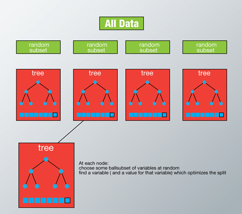
• If there are M input variables, a number m<M is specified such that at each node, m variables are selected at random out of the M. The best split on these m is used to split the node. The value of m is held constant while we grow the forest.
• Each tree is grown to the largest extent possible and there is no pruning.
• Predict new data by aggregating the predictions of the ntree trees (i.e., majority votes for classification, average for regression).

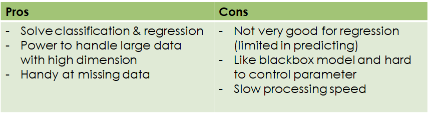
Pros & Cons of Random Forest

ModFit_rf <- train(Ozone~Solar.R+Wind+Temp,data=training,method="rf",prox=TRUE)
predict_rf <- predict(ModFit_rf,testing)                                                            

5.4.7 Train model using Artificial Neural Network

• Formulation of Neural Network

Here, x1,x2....xn are input variables. w1,w2....wn are weights of respective inputs.
b is the bias, which is summed with the weighted inputs to form the net inputs. 
Bias and weights are both adjustable parameters of the neuron.
Parameters are adjusted using some learning rules. 
The output of a neuron can range from -inf to +inf.
The neuron doesn’t know the boundary. So we need a mapping mechanism between the input and output of the neuron. 
This mechanism of mapping inputs to output is known as Activation Function.

• Activation functions:

• Neural Network formulation

• Basic Type of Neural Network:

library(neuralnet)
smax <- apply(training,2,max)
smin <- apply(training,2,min)
trainNN <- as.data.frame(scale(training,center=smin,scale=smax-smin))
testNN <- as.data.frame(scale(testing,center=smin,scale=smax-smin))
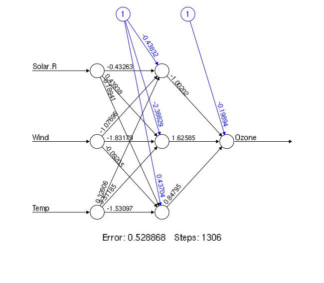
ModNN <- neuralnet(Ozone~Solar.R+Wind+Temp,trainNN, hidden=3,linear.output = T)
plot(ModNN)

predict_ann <- compute(ModNN,testNN)
# Rescale to original:
predict_ann_rescale <- predict_ann$net.result*(smax-smin)[1]+smin[1]

5.5 Evaluate model output

For continuous, we use postResample:

postResample(predict_lm,testing$Ozone)
postResample(predict_SLR,testing$Ozone)
postResample(predict_PCR,testing$Ozone)
postResample(predict_poly,testing$Ozone)
postResample(predict_rpart,testing$Ozone)
postResample(predict_rf,testing$Ozone)
postResample(predict_ann_rescale,testing$Ozone)

Key Points

• Regression training