Fundamental Text Mining using R

Overview

Teaching: 20 min
Exercises: 0 min

Questions

What is Text Mining and how to use R to work with that

Objectives

Learn some terminology in Text Mining with R

11. Text Mining Introduction

We will walk through the Text Mining using an example with Halloween scary monster poem using the most popular Text Mining package tm

Set working directory

rm(list=ls())
setwd('/users/tuev/SMU/Workshop/SMU/R_Text_Mining/')

Opening an example

library(tm)
library(ggplot2)
mytxt <- readLines('https://raw.githubusercontent.com/vuminhtue/SMU_Machine_Learning_R/master/data/monster_mash.txt')

Library tm

A framework for text mining applications within R.The tm package offers

functionality for managing text documents, abstracts the process of document manipulation and eases the usage of heterogeneous text formats in R. The package has integrated database back-end support to minimize memory demands. An advanced meta data management is implemented for collections of text documents to alleviate the usage of large and with meta data enriched document sets.

The package provides native support for reading in several classic file formats (e.g. plain text, PDFs, or XML files).

tm provides easy access to preprocessing and manipulation mechanisms such as whitespace removal, stemming, or stopword deletion. Further a generic filter architecture is available in order to filter documents for certain criteria, or perform full text search. The package supports the export from document collections to term-document matrices.

Corpus Corpora

Corpora are collections of documents containing (natural language) text. In packages which employ the infrastructure provided by package tm, such corpora are represented via the virtual S3 class Corpus: such packages then provide S3 corpus classes extending the virtual base class (such as VCorpus provided by package tm itself).

A corpus can have two types of metadata

# Convert to Corpus format
dc <- VCorpus(VectorSource(mytxt))

Text manipulation

Now that we have converted text data to Corpus format, we can reduce the text dimension using some popular builtin function in tm library

Lower case

Here we enforce that all of the text is lowercase. This makes it easier to match cases and sort words.

Notice we are assigning our modified column back to itself. This will save our modifications to our Data Frame

dc <- tm_map(dc,content_transformer(tolower))
for (i in 1:12) print(dc[[i]]$content)

Remove Punctuation

Here we remove all punctuation from the data. This allows us to focus on the words only as well as assist in matching.

dc <- tm_map(dc,removePunctuation)
for (i in 1:12) print(dc[[i]]$content)

Remove Stopwords

Stopwords are words that are commonly used and do little to aid in the understanding of the content of a text. There is no universal list of stopwords and they vary on the style, time period and media from which your text came from. Typically, people choose to remove stopwords from their data, as it adds extra clutter while the words themselves provide little to no insight as to the nature of the data. For now, we are simply going to count them to get an idea of how many there are.

dc <- tm_map(dc,removeWords,stopwords("english"))
for (i in 1:12) print(dc[[i]]$content)

Strip white space

dc <- tm_map(dc,stripWhitespace)
for (i in 1:12) print(dc[[i]]$content)

Stemming

Stemming is the process of removing suffices, like “ed” or “ing”.

dc_stemmed <- tm_map(dc,stemDocument)
for (i in 1:12) print(dc_stemmed[[i]]$content)

As we can see “eyes” became “eye”, which could help an analysis, but “castle” became “castl” which is less helpful.

Lemmatization

library(textstem)
dc_lemmatize <- tm_map(dc,content_transformer(lemmatize_strings))
for (i in 1:12) print(dc_lemmatize[[i]]$content)

Notice how we still caught “eyes” to “eye” but left “castle” as is.

TermDocumenMatrix

The text data is unstructure data and you need to convert that into structured data for ML analyses. There are two approaches to convert unstructured data to a structured form:

Bag of Words Model
Vector Space Model

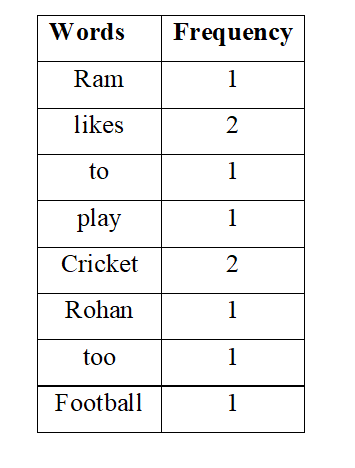
1. Bag of Words model

In the Bag of Words model, the text document is represented by a bag of words. The model can be represented as a table containing the frequency of the words and the words themselves. For instance, consider a text document containing the following sentences-

“Ram likes to play Cricket”
“Rohan likes Cricket too”
“Ram likes Football”

The bag of words for the text document is:

2. Vector Space Model

Vector Space Model (VSM) is the generalization of the Bag of Words model. In the Vector Space model, each document from the corpus is represented as a multidimensional vector. Each unique term from the corpus represents one dimension of the vector space. A term can be a single word or sequence of words (ngrams). The number of unique terms in the corpus determines the dimension of the vector space.

Term Document Matrix

In VSM, the corpus is represented in the form of the Term Document Matrix. Term Document Matrix represents documents vectors in matrix form in which the rows correspond to the terms in the document, columns correspond to the documents in the corpus and cells correspond to the weights of the terms.

Document term matrix

DTM (Document term matrix) is obtained by taking the transpose of TDM. In DTM, the rows correspond to the documents in the corpus and the columns correspond to the terms in the documents and the cells correspond to the weights of the terms.

No we can apply the TF-IDF using control for shorter script Note: We are using the original dc data:

dc_tdm <- TermDocumentMatrix(dc_lemmatize)
print(dc_tdm$dimnames$Terms)

3. Computing Terms’ Weights

There are various approaches for determining the terms’ weights. The simple and frequently used approaches include:-

3.1. Binary weights 3.2. Term Frequency (TF) 3.3. Inverse Document Frequency (IDF) 3.4. Term Frequency-Inverse Document Frequency (TF-IDF)

3.1. Binary weights

In the case of binary weights, the weights take the values- 0 or 1 where 1 reflects the presence and 0 reflects the absence of the term in a particular document. For instance,

D1: Text mining is to find useful information from text. D2: Useful information is mined from the text. D3: Dark came.

3.2. Term Frequency (TF)

In the case of the Term Frequency, the weights represent the frequency of the term in a specific document. The underlying assumption is that the higher the term frequency in a document, the more important it is for that document.

TF(t)= c(t,d) c(t,d)- the number of occurences of the term t in the document d.

3.3. Inverse Document Frequency (IDF)

In the case of IDF, the underlying idea is to assign higher weights to unusual terms, i.e., to terms that are not so common in the corpus. IDF is computed at the corpus level, and thus describes corpus as a whole, not individual documents. It is computed in the following way:

IDF(t)=1+log(N/df(t))

N: number of documents in the corpus Df(t): number of documents with the term t

For instance, suppose there are 100 documents in the corpus and 10 documents contain the term text.

Then, IDF(text)=1+log(100/10)=1+1=2

3.4. TF-IDF

In the case of TF-IDF, the underlying idea is to value those terms that are not so common in the corpus (relatively high IDF), but still have some reasonable level of frequency (relatively high TF). It is the most frequently used metric for computing term weights in a vector space model.

General formula for computing TF-IDF:

TF-IDF(t)=TF(t)*IDF(t)

One popular ‘instantiation’ of this formula:

TF-IDF(t)= tf(t)*log(N/df(t))

Implementing in R code

The following terms are computed using TermDocumentMatrix function

dc_tdm <- TermDocumentMatrix(dc_lemmatize)
print(dc_tdm$dimnames$Terms)

To analyze the term frequency:

CorpusMatrix <- as.matrix(dc_tdm)
sortedMatrix <- sort(rowSums(CorpusMatrix),decreasing=TRUE)
dfCorpus <- data.frame(word = names(sortedMatrix),freq=sortedMatrix)
head(dfCorpus,5)

Bar plot

w <- rowSums(CorpusMatrix)
w_sub <- subset(w,w>3)
barplot(w_sub,las=3, col=rainbow(20))

Word Clouds

library(wordcloud2)
wordcloud2(data=dfCorpus,size=1.6,shape='star')

reate N-Grams and plot histogram using RWeka

library(RWeka)
dfNgrams <- data.frame(text=sapply(dc_lemmatize,as.character),stringsAsFactors = FALSE)
uniGramToken <- NGramTokenizer(dfNgrams,Weka_control(min=1,max=1))
biGramToken <- NGramTokenizer(dfNgrams,Weka_control(min=2,max=2))
triGramToken <- NGramTokenizer(dfNgrams,Weka_control(min=3,max=3))

uniGrams <- data.frame(table(uniGramToken))
biGrams  <- data.frame(table(biGramToken))
triGrams <- data.frame(table(triGramToken))

uniGrams <- uniGrams[order(uniGrams$Freq,decreasing=TRUE),]
colnames(uniGrams) <- c('Word','Frequency')
biGrams <- biGrams[order(biGrams$Freq,decreasing=TRUE),]
colnames(biGrams) <- c('Word','Frequency')
triGrams <- triGrams[order(triGrams$Freq,decreasing=TRUE),]
colnames(triGrams) <- c('Word','Frequency')

uniGrams_s <- uniGrams[1:10,]
biGrams_s  <- biGrams[1:10,]
triGrams_s <- triGrams[1:10,]

library(ggplot2)
plotUniGrams <- ggplot(head(uniGrams,10),aes(x=Frequency,y=reorder(Word,Frequency),fill=Word))+
                  geom_bar(stat='identity')+
                  scale_fill_brewer(palette="Spectral")+
                  geom_text(aes(x=Frequency,label=Frequency,vjust=1))+
                  labs(x="Frequency (%)",y="Words",title="UniGrams Frequency")
                  
                  
plotUniGrams

plotBiGrams <- ggplot(head(biGrams,10),aes(x=Frequency,y=reorder(Word,Frequency),fill=Word))+
                  geom_bar(stat='identity')+
                  scale_fill_brewer(palette="Spectral")+
                  geom_text(aes(x=Frequency,label=Frequency,vjust=1))+
                  labs(x="Frequency (%)",y="Words",title="BiGrams Frequency")
plotBiGrams

plotTriGrams <- ggplot(head(triGrams,10),aes(x=Frequency,y=reorder(Word,Frequency),fill=Word))+
                  geom_bar(stat='identity')+
                  scale_fill_brewer(palette="Spectral")+
                  geom_text(aes(x=Frequency,label=Frequency,vjust=1))+
                  labs(x="Frequency (%)",y="Words",title="TriGrams Frequency")
plotTriGrams

Word Clouds for BiGrams and TriGrams

wordcloud2(data=uniGrams,size=1.6)
wordcloud2(data=biGrams,size=1.6)
wordcloud2(data=triGrams,size=1.6)

Exercise

DATA

For this comparison, our data set is a sample of 19 documents from the Gutenberg Collection. The Project Gutenberg is a volunteer effort to digitize and archive cultural works as well as to “encourage the creation and distribution of eBooks”, found in 1971 and is the oldest digital library.

The Gutenberg collection can be accessed in R using the “gutenbergr” package.

The data for this example is a data frame with four columns and nineteen rows. Each row represents a document. The text of the document is in the full_text variable. The remaining columns - id, author, and title - provide metadata for the given document.

The gutenbergr package provides access to the public domain works from the Project Gutenberg collection. The package includes tools both for downloading books (stripping out the unhelpful header/footer information), and a complete dataset of Project Gutenberg metadata that can be used to find works of interest. In this book, we will mostly use the function gutenberg_download() that downloads one or more works from Project Gutenberg by ID, but you can also use other functions to explore metadata, pair Gutenberg ID with title, author, language, etc., or gather information about authors.

Let see how many authors and subjects in Gutenberg collection?

library(gutenbergr)
#List first 10 authors
gutenberg_authors$author[1:10]

#List first 10 subjects:
gutenberg_subjects$subject[1:10]

Create the collections of books by author Jane Austen

books <- gutenberg_works(author == "Austen, Jane")
dim(books)

A tibble is a modern class of data frame within R, available in the dplyr and tibble packages, that has a convenient print method, will not convert strings to factors, and does not use row names. Tibbles are great for use with tidy tools.

The dimension of books is (10,8) with 10 rows and 8 cols.

Each col is a meta data:

colnames(books)
print(books)

Each book title is has its own id and we can access the content of each book via downloading its id

book_105_121 <- gutenberg_download(c(105,121))

Now we can see that the tible book_105_121 is created and it has shape of 16319 rows with 2 cols: id and text. The IDs have only 2 values 105 and 121 and the text is the content of the selected book’s ID

print(dim(book_105_121))
head(book_105_121$text,20)

Now we will go into detail of text mining for this book by Jane Austen.

For simplicity, we use only book id 105 for our analyses:

book_105 <- gutenberg_download(105)

Convert the tible data to Corpus format for use in tm library

mydc <- VCorpus(VectorSource(book_105$text))

Manipulate the data

mydc <- tm_map(mydc,content_transformer(tolower))
mydc <- tm_map(mydc,removePunctuation)
mydc <- tm_map(mydc,removeWords,stopwords("english"))
mydc <- tm_map(mydc,stripWhitespace)
mydc <- tm_map(mydc,PlainTextDocument)
mydc_lemmatize <- tm_map(mydc,content_transformer(lemmatize_strings))

Calculte term frequency on the Corpus data

mydc_tdm <- TermDocumentMatrix(mydc)
CorpusMatrix <- as.matrix(mydc_tdm)
sortedMatrix <- sort(rowSums(CorpusMatrix))
dfCorpus <- data.frame(word = names(sortedMatrix),freq=sortedMatrix)
wordcloud2(data=dfCorpus,size=1.6)

library(RWeka)
dfNgrams <- data.frame(text=sapply(mydc,as.character),stringsAsFactors = FALSE)
uniGramToken <- NGramTokenizer(dfNgrams,Weka_control(min=1,max=1))
biGramToken <- NGramTokenizer(dfNgrams,Weka_control(min=2,max=2))
triGramToken <- NGramTokenizer(dfNgrams,Weka_control(min=3,max=3))

uniGrams <- data.frame(table(uniGramToken))
biGrams  <- data.frame(table(biGramToken))
triGrams <- data.frame(table(triGramToken))

uniGrams <- uniGrams[order(uniGrams$Freq,decreasing=TRUE),]
colnames(uniGrams) <- c('Word','Frequency')
biGrams <- biGrams[order(biGrams$Freq,decreasing=TRUE),]
colnames(biGrams) <- c('Word','Frequency')
triGrams <- triGrams[order(triGrams$Freq,decreasing=TRUE),]
colnames(triGrams) <- c('Word','Frequency')

plotUniGrams <- ggplot(head(uniGrams,10),aes(x=Frequency,y=reorder(Word,Frequency),fill=Word))+
                  geom_bar(stat='identity')+
                  scale_fill_brewer(palette="Spectral")+
                  geom_text(aes(x=Frequency,label=Frequency,vjust=1))+
                  labs(x="Frequency (%)",y="Words",title="UniGrams Frequency")
                  
                  
plotUniGrams

plotBiGrams <- ggplot(head(biGrams,10),aes(x=Frequency,y=reorder(Word,Frequency),fill=Word))+
                  geom_bar(stat='identity')+
                  scale_fill_brewer(palette="Spectral")+
                  geom_text(aes(x=Frequency,label=Frequency,vjust=1))+
                  labs(x="Frequency (%)",y="Words",title="BiGrams Frequency")
                  
                  
plotBiGrams

plotTriGrams <- ggplot(head(triGrams,10),aes(x=Frequency,y=reorder(Word,Frequency),fill=Word))+
                  geom_bar(stat='identity')+
                  scale_fill_brewer(palette="Spectral")+
                  geom_text(aes(x=Frequency,label=Frequency,vjust=1))+
                  labs(x="Frequency (%)",y="Words",title="TriGrams Frequency")
                  
                  
plotTriGrams

wordcloud2(uniGrams,size=1.6)

wordcloud2(biGrams,size=1.6)

wordcloud2(triGrams,size=1.6)

Key Points

Text Mining, R

previous episode

Machine Learning with R

next episode