Regularization and Variable Selection

Overview

Teaching: 20 min
Exercises: 0 min

Questions

• Why do we need Regularization and Variable Selection in ML model

Objectives

• Learn how to apply Regularization and Variable selection in ML model

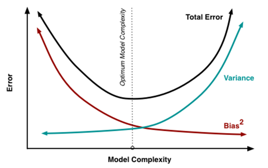
• One of the major aspects of training your machine learning model is to avoid overfitting (Using more parameter to best fit the training but on the other hand, failed to evaluate the testing).
• The concept of balancing bias and variance, is helpful in understanding the phenomenon of overfitting

8.1 Regularization

• In order to reduce the Model Complexity or to avoid Multi-Collinearity, one needs to reduce the number of covariates (or set the coefficient to be zero).
• If the coefficients are too large, let’s penalize them to enforce them to be smaller
• Regularization is a form of multilinear regression, that constrains/regularizes or shrinks the coefficient estimates towards zero.
• In other words, this technique discourages learning a more complex or flexible model, so as to avoid the risk of overfitting
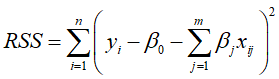
• A simple Multi-Linear Regression look like this:

=> in which: β represents the coefficient estimates for different variables or predictors(x)

The residual sum of squares RSS is the loss function of the fitting procedure. And we need to determine the optimal coefficients 𝛽 to minimize the loss function

This procedure will adjust the β based on the training data. If there is any noise in training data, the model will not perform well for testing data. Thus, Regularization comes in and regularizes/shrinkage these 𝛽 towards zero.

There are 3 main types of Regularization.

• Ridge Regression
• LASSO
• Elastics Nets

For simplicity, I only introduce LASSO for Regularization method

LASSO: Least Absolute Shrinkage & Selection Operator

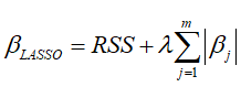
• In order to overcome the cons issue in Ridge Regression, the LASSO is introduced with the similar shrinkage parameter, but the different is not in square term of the coefficient but only absolute value
• Similar to Ridge Regression, LASSO also shrink the coefficient, but force coefficients to be equal to 0. Making it ability to perform feature selection
• In statistics the coefficient esimated produced by this method is know as L1 norm

Setting up training/testing model:

library(caret)
#library(ElemStatLearn)=> available for R package > 3.6.2
prostate=read.csv("https://raw.githubusercontent.com/vuminhtue/Machine-Learning-Python/master/data/prostate_data.csv")


set.seed(123)
indT <- which(prostate$train==TRUE)
training <- prostate[indT,]
testing  <- prostate[-indT,]

library(PerformanceAnalytics)
chart.Correlation(training[,-10])

Splitting to training/testing

library(glmnet)
library(plotmo)
y <- training$lpsa
x <- training[,-c(9,10)]
x <- as.matrix(x)

LASSO computation

cvfit_LASSO    <- cv.glmnet(x,y,alpha=1)
plot(cvfit_LASSO)

log(cvfit_LASSO$lambda.min)
log(cvfit_LASSO$lambda.1se)

coef(cvfit_LASSO,s=cvfit_LASSO$lambda.min)
coef(cvfit_LASSO,s=cvfit_LASSO$lambda.1se)

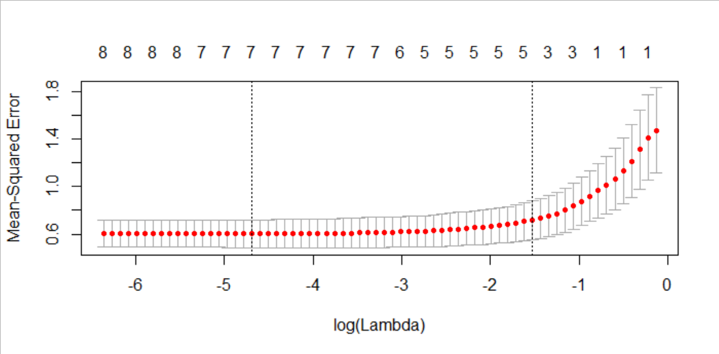
• The plot shows the Mean Square Error based on training model with 𝜆 variation.
• Top of the chart shows number of predictors used. Now instead of showing all 8 predictors as in Ridge Regression, LASSO shows the different number of predictors as MSE values change.
• Similar to RR, there are 2 𝜆 values: (1) 𝜆.min which can be computed using log(cvfit_LASSO$lambda.min) and (2) 𝜆.1se (1 standard error from min value) which can be computed using log(cvfit_LASSO$lambda.1se)
• The corresponding β values for each predictors can be found using coef(cvfit_Ridge,s=cvfit_LASSO$lambda.1se) or coef(cvfit_LASSO,s=cvfit_Ridge$lambda.min)

Fit_LASSO <- glmnet(x,y,alpha=1)
plot_glmnet(Fit_LASSO,label=TRUE,xvar="lambda",
            col=seq(1,8),,grid.col = 'lightgray')

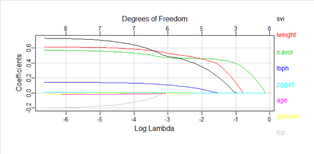The plot shows different coefficients for all predictors with 𝜆 variation. Depending on 𝜆 values that the β varying and it can be 0 at certain point.

Using 𝜆.1se, we obtain reasonable result:

> predict_LASSO <- predict(cvfit_LASSO,newx=xtest,s="lambda.1se")
> postResample(predict_LASSO,testing$lpsa)
     RMSE  Rsquared       MAE 
0.6783357 0.6096333 0.5030956 

8.2 Dimension Reduction using PCA

• Handy with large data
• Where many variables correlate with one another, they will all contribute strongly to the same principal component
• Each principal component sums up a certain percentage of the total variation in the dataset
• More Principal Components, more summarization of the original data sets

8.2.1 Explanation

• For example, we have 3 data sets: X, Y, Z
• We need to compute the covariance matrix M for the 3 data set:

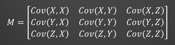
in which, the covariance value between 2 data sets can be computed as:

• For the Covariance matrix M, we will find m eigenvectors and m eigenvalues

- Given mxm matrix, we can find m eigenvectors and m eigenvalues
- Eigenvectors can only be found for square matrix.
- Not every square matrix has eigenvectors
- A square matrix A and its transpose have the same eigenvalues but different eigenvectors
- The eigenvalues of a diagonal or triangular matrix are its diagonal elements.
- Eigenvectors of a matrix A with distinct eigenvalues are linearly independent.

Eigenvector with the largest eigenvalue forms the first principal component of the data set … and so on …*

8.2.2 Implementation

8.2.2.1 Compute PCA using eigenvector:

library(PerformanceAnalytics)
data(mtcars)
#Ignore vs & am (PCA works good with numeric data )
datain <- mtcars[,c(1:7,10:11)]
chart.Correlation(datain)
cin <- cov(scale(datain))
ein <- eigen(cin)
newpca <-   -scale(datain) %*% ein$vectors

8.2.2.2 Compute PCA using built-in function:

mtcars.pca <- prcomp(datain,center=TRUE,scale=TRUE)
summary(mtcars.pca)

8.2.2.3 A nice way to plot PCA:

Install ggbiplot package:

library(devtools)
install_github("vqv/ggbiplot")

library(ggbiplot)
ggbiplot(mtcars.pca)
ggbiplot(mtcars.pca, labels=rownames(mtcars))
ggbiplot(mtcars.pca,ellipse=TRUE,  labels=rownames(mtcars))

mtcars.country <- c(rep("Japan", 3), rep("US",4), rep("Europe", 7),rep("US",3), "Europe", rep("Japan", 3), rep("US",4), rep("Europe", 3), "US", rep("Europe", 3))

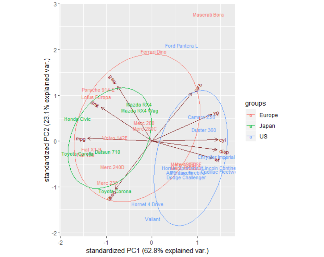
ggbiplot(mtcars.pca,ellipse=TRUE,labels=rownames(mtcars),groups = mtcars.country)

8.2.2.4 Application of PCA model in Machine Learning:

data(mtcars)
set.seed(123)
datain <- mtcars[,c(1:7,10:11)]

indT <- createDataPartition(y=datain$mpg,p=0.6,list=FALSE)
training <- datain[indT,]
testing  <- datain[-indT,]

preProc <- preProcess(training[,-1],method="pca",pcaComp = 1)
trainPC <- predict(preProc,training[,-1])
testPC  <- predict(preProc,testing[,-1])

traindat<- cbind(training$mpg,trainPC)
testdat <- cbind(testing$mpg,testPC)

names(traindat) <- c("mpg","PC1")
names(testdat)  <- names(traindat) 

modFitPC<- train(mpg~.,method="lm",data=traindat)

predictand <- predict(modFitPC,testdat)
postResample(testing$mpg,as.vector(predictand))

Key Points

• Regularization, Ridge Regression, LASSO, Elastic Nets, PCA