Training Machine Learning model using Regression Method

Overview

Teaching: 20 min
Exercises: 0 min

Questions

How to train a Machine Learning model using Regression method

Objectives

Learn to use different Regression algorithm for Machine Learning training

5 Supervised Learning training with Regression

5.1 For continuous output

5.1.1 Train model using Linear Regression with 1 predictor

Let use the airquality data in previous episodes:

import pandas as pd
import numpy as np
from sklearn.impute import KNNImputer
from sklearn.model_selection import train_test_split
from sklearn import metrics

data_df = pd.DataFrame(pd.read_csv('https://raw.githubusercontent.com/vuminhtue/Machine-Learning-Python/master/data/r_airquality.csv'))

imputer = KNNImputer(n_neighbors=2, weights="uniform")
data_knnimpute = pd.DataFrame(imputer.fit_transform(data_df))
data_knnimpute.columns = data_df.columns

X_train, X_test, y_train, y_test = train_test_split(data_knnimpute['Temp'],
                                                    data_knnimpute['Ozone'],
                                                    train_size=0.6,random_state=123)

Fit a Linear model using method=lm

from sklearn.linear_model import LinearRegression
model_linreg = LinearRegression().fit(X_train[:,None],y_train)

Apply trained model to testing data set and evaluate output using R-squared:

y_pred = model_linreg.predict(X_test[:,None])
metrics.r2_score(y_test,y_pred) # R^2
metrics.mean_squared_error(y_test,y_pred,squared=False) #RMSE

5.1.2 Train model using Multi-Linear Regression (with 2 or more predictors)

From the above model, the R2=0.39:

The reason is that we only build the model with 1 input Temp. In this section, we will build the model with more input Solar Radiation, Wind, Temperature:

X_train, X_test, y_train, y_test = train_test_split(data_knnimpute[['Temp','Wind','Solar.R']],
                                                    data_knnimpute['Ozone'],
                                                    train_size=0.6,random_state=123)
model_linreg = LinearRegression().fit(X_train,y_train)
y_pred2 = model_linreg.predict(X_test)

metrics.r2_score(y_test,y_pred2)
metrics.mean_squared_error(y_test,y_pred2,squared=False)

Output is therefore better with smaller RMSE and higher Rsquared at 0.5

5.1.3 Train model using Polynomial Regression

From Multi-Linear Regression, the best R2=0.5 using 3 predictors. We can slightly improve this by using Polynomial Regression

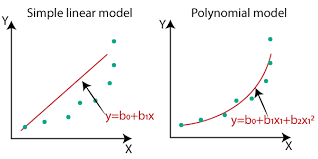
In this study, let use polynomial regression with degree of freedom=2

from sklearn.preprocessing import PolynomialFeatures
poly = PolynomialFeatures(degree=2)
X_train_poly = poly.fit_transform(data_knnimpute[['Temp','Wind','Solar.R']])
X_train, X_test, y_train, y_test = train_test_split(X_train_poly,
                                                    data_knnimpute['Ozone'],
                                                    train_size=0.6,random_state=123)
model_linreg_poly = LinearRegression().fit(X_train,y_train)
y_pred_poly = model_linreg_poly.predict(X_test)
print(metrics.r2_score(y_test,y_pred_poly))
print(metrics.mean_squared_error(y_test,y_pred_poly,squared=False))

The R2=0.58 shows improvement using polynomial regression!

5.2 For categorical output

5.2.1 Train model using Logistic Regression

Logistic regression is another technique borrowed by machine learning from the field of statistics. It is the go-to method for binary classification problems (problems with two class values).
Typical binary classification: True/False, Yes/No, Pass/Fail, Spam/No Spam, Male/Female
Unlike linear regression, the prediction for the output is transformed using a non-linear function called the logistic function.
The standard logistic function has formulation:

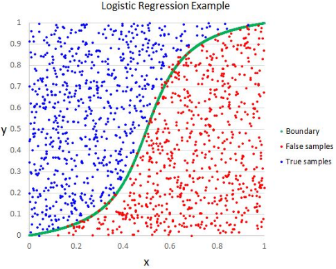
In this example, we create a sample data set and use logistic regression to solve it. The example is taken from here

Load library and create sample data set:

from sklearn.datasets import make_classification

# generate sample data
X, y = make_classification(n_samples=1000, n_classes=2, random_state=1)

Partitioning Data to train/test:

from sklearn.model_selection import train_test_split
X_train, X_test, y_train, y_test = train_test_split(X, y, test_size=0.5, random_state=2)

Train model using Logistic Regression

from sklearn.linear_model import LogisticRegression
model_LogReg = LogisticRegression().fit(X_train, y_train)
y_pred = model_LogReg.predict(X_test)

from sklearn.linear_model import LogisticRegression
model_LogReg = LogisticRegression().fit(X_train, y_train)
# predict output:
y_pred = model_LogReg.predict(X_test)
# predict probabilities
lr_probs = model_LogReg.predict_proba(X_test)

Evaluate output with accurary level:

from sklearn import metrics
metrics.accuracy_score(y_test,y_pred)

We retrieve the accuracy = 0.834

Now compute AUC-ROC and plot curve

from sklearn.metrics import roc_curve, roc_auc_score
import matplotlib.pyplot as plt
import numpy as np

# generate a no skill prediction (majority class)
ns_probs = np.zeros(len(y_test))

# calculate scores
ns_auc = roc_auc_score(y_test, ns_probs)
lr_auc = roc_auc_score(y_test, lr_probs[:,1])
# summarize scores
print('No Skill: ROC AUC=%.3f' % (ns_auc))
print('Logistic: ROC AUC=%.3f' % (lr_auc))
# calculate roc curves
ns_fpr, ns_tpr, _ = roc_curve(y_test, ns_probs)
lr_fpr, lr_tpr, _ = roc_curve(y_test, lr_probs[:,1])
# plot the roc curve for the model
plt.plot(ns_fpr, ns_tpr, linestyle='--', label='No Skill')
plt.plot(lr_fpr, lr_tpr, marker='.', label='Logistic')
# axis labels
plt.xlabel('False Positive Rate')
plt.ylabel('True Positive Rate')
# show the legend
plt.legend()
# show the plot
plt.show()

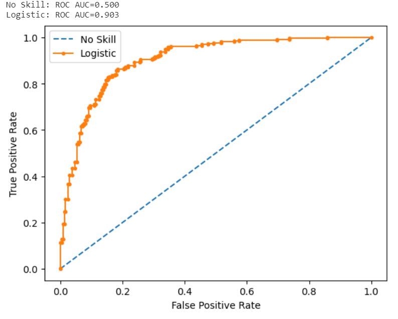
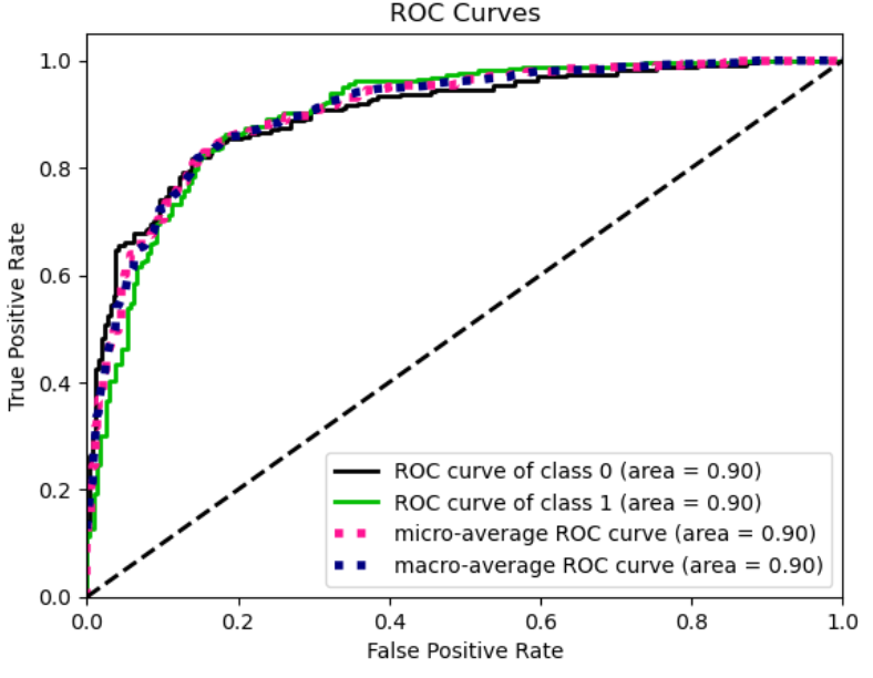
An alternative way to plot AUC-ROC curve, using additional toolbox “scikit-plot”

pip install scikit-plot

The shorter code for using this library:

import scikitplot as skplt
skplt.metrics.plot_roc(y_test, lr_probs)
plt.show()

Key Points

Regression training

previous episode

Introduction to Machine Learning using Python

next episode