Dimension Reduction
Overview
Teaching: 20 min
Exercises: 0 minQuestions
What happen when there are lots of covariates?
Objectives
Learn how to apply PCA in ML model
10 Principal Component Analysis
- Handy with large data
- Where many variables correlate with one another, they will all contribute strongly to the same principal component
- Each principal component sums up a certain percentage of the total variation in the dataset
- More Principal Components, more summarization of the original data sets
10.1 PCA formulation
- For example, we have 3 data sets:
X, Y, Z - We need to compute the covariance matrix M for the 3 data set:
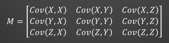
in which, the covariance value between 2 data sets can be computed as:
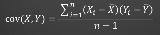
- For the Covariance matrix M, we will find m eigenvectors and m eigenvalues
- Given mxm matrix, we can find m eigenvectors and m eigenvalues
- Eigenvectors can only be found for square matrix.
- Not every square matrix has eigenvectors
- A square matrix A and its transpose have the same eigenvalues but different eigenvectors
- The eigenvalues of a diagonal or triangular matrix are its diagonal elements.
- Eigenvectors of a matrix A with distinct eigenvalues are linearly independent.
Eigenvector with the largest eigenvalue forms the first principal component of the data set … and so on …*
10.2 Implementation
Here we gonna use iris data set:
from sklearn.datasets import load_iris
from sklearn.model_selection import train_test_split
from sklearn.preprocessing import StandardScaler

import numpy as np
import pandas as pd
iris = load_iris()
X = iris.data
y = pd.DataFrame(iris.target)
y['Species']=pd.Categorical.from_codes(iris.target, iris.target_names)
X_train, X_test, y_train, y_test = train_test_split(X,y,train_size=0.6,random_state=123)

X_train_scaled = StandardScaler().fit_transform(X_train)
X_test_scaled = StandardScaler().fit_transform(X_test)
10.2.1 Compute PCA using sklearn:
from sklearn.decomposition import PCA
pca = PCA(n_components=4)
PCs = pca.fit_transform(X_train_scaled)
PCs = pd.DataFrame(PCs,columns = ['PC1','PC2','PC3','PC4'])
We can see that PCs computed from sklearn package are similar to newpca computed from using eigen vectors
10.2.2 Explained Variance
The explained variance tells you how much information (variance) can be attributed to each of the principal components.
pca.explained_variance_ratio_
In this example: the PC1(0.74) and PC2 (0.21) consume 0.95 percent of explained variance. Therefore, using 2 Principal Components should be good enough
10.2.3 Application of PCA model in Machine Learning:
from sklearn.ensemble import RandomForestClassifier
from sklearn.metrics import accuracy_score as acc_score

pca = PCA(n_components=2) #We choose number of principal components to be 2

X_train_pca = pca.fit_transform(X_train_scaled)
X_test_pca = pd.DataFrame(pca.transform(X_test_scaled))
X_test_pca.columns=['PC1','PC2']

print(pca.explained_variance_ratio_)

# Use random forest to train model
model_RF = RandomForestClassifier(n_estimators=20,criterion="gini",random_state=1234).fit(X_train_pca, y_train['Species'])
y_pred_RF = model_RF.predict(X_test_pca)
acc_score(y_test['Species'],y_pred_RF)
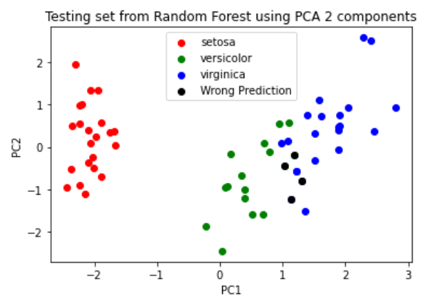
Plotting the testing result with indicator of Wrong prediction
import matplotlib.pyplot as plt

ax = plt.gca()

targets = np.unique(y_pred_RF)
colors = ['r', 'g', 'b']

for target, color in zip(targets,colors):
    indp = y_pred_RF == target
    ax.scatter(X_test_pca.loc[indp, 'PC1'], X_test_pca.loc[indp, 'PC2'],c = color)

# Ploting the Wrong Prediction
ind = y_pred_RF!=np.array(y_test['Species'])
ax.scatter(X_test_pca.loc[ind, 'PC1'],X_test_pca.loc[ind, 'PC2'],c = 'black')

#axis control
ax.legend(['setosa','versicolor','virginica','Wrong Prediction'])
ax.set_title("Testing set from Random Forest using PCA 2 components")
ax.set_xlabel('PC1')
ax.set_ylabel('PC2')

plt.show()
Key Points
PCA