Support Vector Machine

Overview

Teaching: 20 min
Exercises: 0 min

Questions

• How to use Support Vector Machine in Machine Learning model

Objectives

• Learn how to use SVM in ML model

12. Support Vector Machine

• A support vector machine is a very important and versatile machine learning algorithm,
• It is capable of doing linear and nonlinear classification, regression and outlier detection.
• It is preferred over other classification algorithms because it uses less computation and gives notable accuracy.
• It is good because it gives reliable results even if there is less data
• The objective of the support vector machine (SVM) algorithm is to find a hyperplane in an N-dimensional space that distinctly classifies the data points.

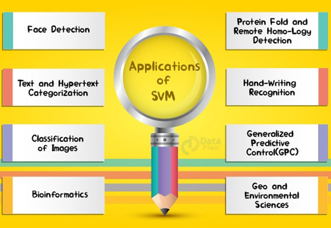
12.1. Applications of Support Vector Machine:

12.2. Explanation

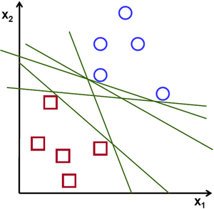
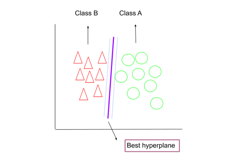
• To separate the two classes of data points, there are many possible hyperplanes that could be chosen

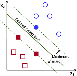
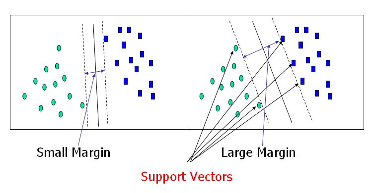
• SVM’s objective is to find a plane that has the maximum margin, i.e the maximum distance between data points of both classes. Maximizing the margin distance provides some reinforcement so that future data points can be classified with more confidence.

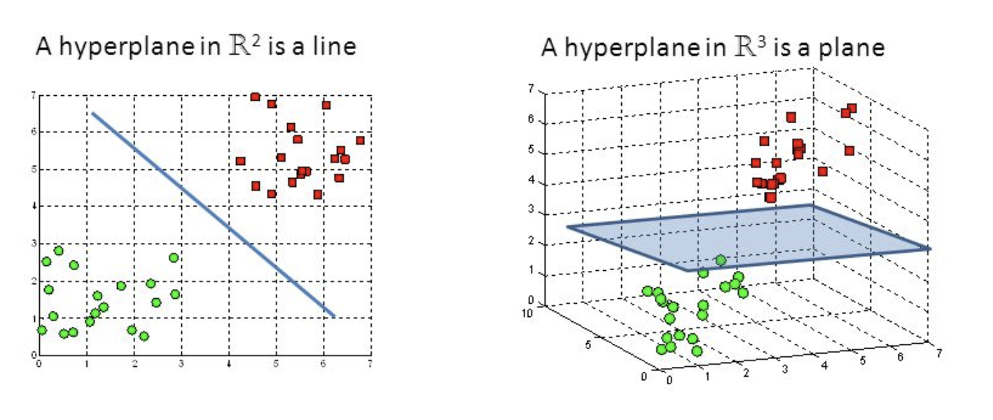
• Example of hyperplane in 2D and 3D position:

• Support vectors (SVs) are data points that are closer to the hyperplane and influence the position and orientation of the hyperplane. Using SVs to maximize the margin of the classifier. Removing SVs will change the position of the hyperplane. These are the points that help us build our SVM.

12.3. SVM’s kernel

12.3.1. For linear separable data, it is quite straight forward to create a hyperplane to distinguish them

12.3.2. For linearly non-separable data, SVM makes use of kernel tricks to make it linearly separable.

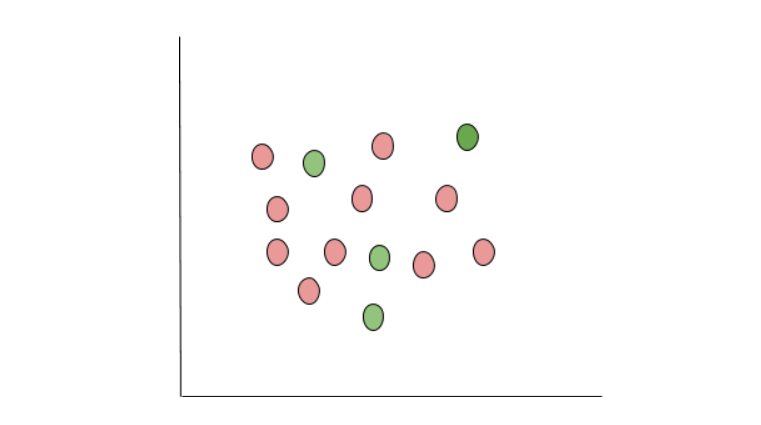
• The concept of transformation of non-linearly separable data into linearly separable is called Cover’s theorem - “given a set of training data that is not linearly separable, with high probability it can be transformed into a linearly separable training set by projecting it into a higher-dimensional space via some non-linear transformation”.
• Kernel tricks help in projecting data points to the higher dimensional space by which they became relatively more easily separable in higher-dimensional space.
• Kernel tricks also known as Generalized dot product.
• Kernel tricks are the way of calculating dot product of two vectors to check how much they make an effect on each other.
• According to Cover’s theorem the chances of linearly non-separable data sets becoming linearly separable increase in higher dimensions.
• Kernel functions are used to get the dot products to solve SVM constrained optimization.

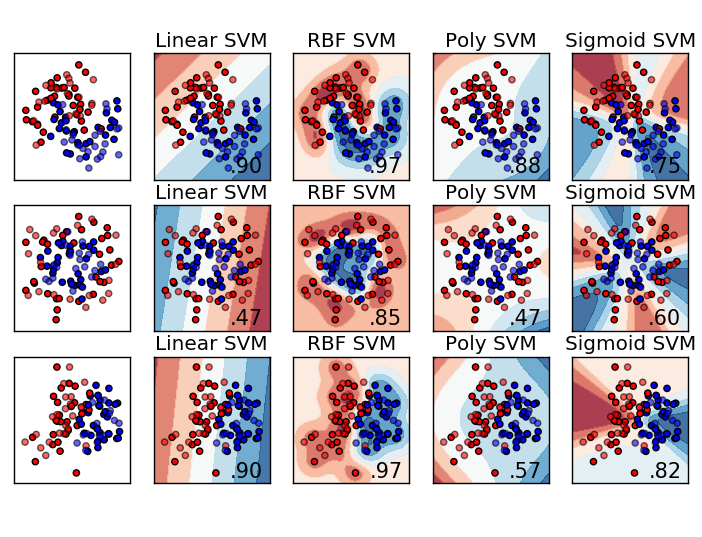
The following kernel trick compared different kernel ‘linear’ , ’poly’ , ‘rbf’ , ‘sigmoid’:

12.4. Implementation

Here we use the regular iris dataset with Classification problem

from sklearn.datasets import load_iris
from sklearn.model_selection import train_test_split
from sklearn.preprocessing import MinMaxScaler

import numpy as np
import pandas as pd
iris = load_iris()
X = iris.data
X = X[:,2:4]
y = iris.target

X_train, X_test, y_train, y_test = train_test_split(X,y,train_size=0.6,random_state=123)

Fit Support Vector Classifier model

from sklearn.svm import SVC
from mlxtend.plotting import plot_decision_regions
import matplotlib.pyplot as plt
names = ["Linear SVM", "RBF SVM", "Poly SVM", "Sigmoid SVM"]
classifiers = [
    SVC(kernel="linear"),
    SVC(kernel="rbf"),
    SVC(kernel="poly"),
    SVC(kernel="sigmoid")]

i = 1
figure = plt.figure(figsize=(27, 5))
cm = plt.cm.jet

for name, clf in zip(names, classifiers):
    ax = plt.subplot(1,4, i)
    clf.fit(X_train, y_train)
    ax = plot_decision_regions(X=X_train, 
                      y=y_train,
                      clf=clf)
    ax.set_xlabel(iris.feature_names[2], size=14)
    ax.set_ylabel(iris.feature_names[3], size=14)
    ax.set_title(name, size=20)
    handles, labels = ax.get_legend_handles_labels()
    ax.legend(handles,iris.target_names)
    i+=1
plt.show()

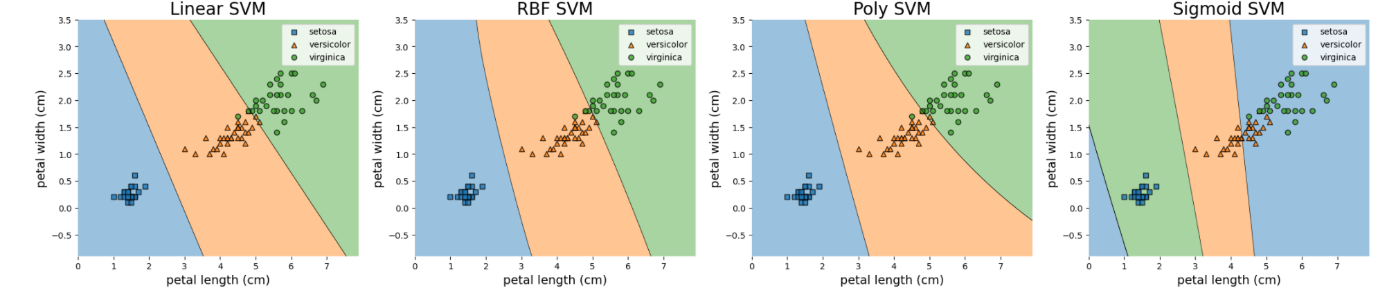
In this model, C is the regularization parameter Default C=1. The strength of the regularization is inversely proportional to C. Must be strictly positive.

12.5. Tips on using SVM

• Setting C=1 is reasonable choice for default. If you have a lot of noisy observations you should decrease it: decreasing C corresponds to more regularization.
• More information here

12.6. Pros of SVM

• High stability due to dependency on support vectors and not the data points.
• Does not get influenced by Outliers.
• No assumptions made of the datasets.
• Numeric predictions problem can be dealt with SVM.

12.7. Cons of SVM

• Blackbox method.
• Inclined to overfitting method.
• Very rigorous computation.

Key Points

• SVM